Machine Learning for Fluid Mechanics

저자: Steven J. Brunton, Bernd R. Noack, and Petros Koumoutsakos

키워드: 머신 러닝, 데이터 기반 모델링, 최적화, 통제(control)

출처: Annual Review of FLuid Mechanics (Volume 52, 2020)

https://www.annualreviews.org/docserver/fulltext/fluid/52/1/annurev-fluid-010719-060214.pdf?expires=1732327852&id=id&accname=guest&checksum=640B7B2D749973FC0F6C8251F72C3B4A

0. 초록

The field of fluid mechanics is rapidly advancing, driven by unprecedented volumes of data from experiments, filed measurements, and large-scale simulateions at multiple spatiotemporal scales. Machine learning(ML) offers a wealth of techniques to extract information from data that can be translated into knowledge about the underlying fluid mechanics. Moreover, ML algorithms can augment domain knowledge and automate tasks related to flow control and optimization. This article presents an overview of past history, current developments, and emerging opportunities of ML for fluid mechanics. We outline fundamental ML methologies and discuss their uses for understanding, modeling, optimizing, and controlling fluid flows. The strength and limitations of these methods are addressed form the perspective of scientific inquiry that considers data as an inherent part of modeling, experiemtns, and simulation. ML provides a powerful information-procession framework that can augment, and possibly even transform, current lines of fluid mecanics research and industrial applications.

유체역학 분야는 실험이나 현장 측정, 그리고 다양한 시공간적 규모에서 이루어지는 대규모 시뮬레이션으로부터 방대한 양을 기반으로 빠르게 발전하고 있다. 머신러닝(ML)은 이러한 데이터를 통해 유체역학에 숨겨져있는 정보를 추출하고 이를 기반으로 유체역학의 근본적인 메커니즘에 대한 지식을 빼올 수 있는 다양한 기법을 제공한다. 또한, ML 알고리즘은 이러한 영역적 지식을 보완하고 흐름 통제나 최적화 같은 기술을 자동화할 수 있게 한다.

이 글에서는 유체역학에서의 ML의 역사와 최근 발전, 그리고 기대되는 전망에 대해 다루고 있다. 여기선 기본적인 ML 방법론을 소개하고, 이것을 어떻게 사용해서 유체역학을 이해하고, 만들고, 최적화시키고, 통제할 수 있는지에 대해 논의할 것이다. 아울러, 이러한 방법들의 장점과 한계점은 과학적 탐구의 관점에서 검토되어질 것이며, 데이터를 모델링과 실험, 그리고 시뮬레이션의 본질적인 일부로 간주할 것이다.

ML은 지금의 유체역학 연구나 산업적 응용을 보완하고 어쩌면 변혁을 일으킬 수도 있는 강력한 정보 처리 프레임위크를 제공한다. 

1. 서론

Fluid mechanics has traditionally dealt with massive amounts of data from experiments, filed measurements, and large-scale numerical simulations. Indeed, in the past few decades, big data have been a reality in fluid mecanics research (Pollard et al. 2016) due to high-performance computing architectures and advances in experimental measurement capabilities. Over the past 50 years, many techniques were developed to handle such data, ranging from advanced algorithms for data processing and compression to fluid mechanics databases (Perlman et al. 2007, Wu & Moin 2008). However, the analysis of fluid mechanics data has relied, to a large extent, on domain expertise, statistical analysis, and heuristic algorithms.

유체역학은 전통적으로 실험이나 현장 측정, 그리고 대규모 시뮬레이션에서 발생하는 방대한 양의 데이터를 다루어 왔다. 실제로 최근 몇십 년 동안, 고성능의 계산 방법과 실험적 측정능력이 발전해감에 따라 방대한 데이터야말로 유체역학의 실체였다. 지난 50년간, 그러한 데이터를 다루기 위한 기술들, 예를 들면 정보 처리나 압축을 위한 고급 알고리즘이나 유체역학 데이터베이스의에 이르기까지 다양한 접근법이 발전되었다. 하지만 유체역학을 특정 분양 전문가의 지식이나 통계 분석, 그리고 휴리스틱(경험적) 알고리즘에 크게 의존해 왔다. 

The growth of data today is widespread across scientific disciplines, and gaining insight and actionalble information from data has become a new mode of scientific inquiry as well as a commercial opportunity. Our generation is experiencing and unprecedented confluence of (a) vast and increasing volumes of data; (b) advances in computational hardware and reduced costs for computation, data storage, and transfer; (c) sophisticated algorithms; (d) an abundance of open source software and benchmark problems; and (e) significant and ongiong investment by industry on data-driven problem solving. These advances have, in turn, fueled renewed interest and progress in the field of machine learning(ML) to extract information from these data. ML is now rapidly making inroads in fluid mechanics. These learning algorithms may be categorized into supervised, semisupervised, and unsupervised learning (see Figure 1), depending in the information available about the data to the learning machine(LM).

과학 전 분야에 걸쳐서 데이터의 증가는 광번위하게 나타나고 있고, 데이터를 통해 통찰력과 활용가능한 정보를 얻는것이 새로운  과학 탐구 방식이나 산업적 기회로 자리 잡게 되었다. 우리 세대는 다음과 같은 전례없는 합류를 경험하고 있다:

(a) 방대하고 점점 더 늘어나는 양의 데이터

(b) 컴퓨터 하드웨어의 발전과 계산, 데이터 저장, 그리고 정보 공유에 대한 비용의 감소

(c) 정교한 알고리즘

(d) 넘쳐나는 오픈소스 소프트웨어와 벤치마크 문제

(e) 데이터 관련 문제해결에 대한 기업들의 끊임없는 투자.

이러한 발전들로 인해 데이터에서 정보를 추출하는 ML 분야에 대한 관심와 발전이 다시 한번 생겨나기 시작했다. ML은 최근 빠르게 유체역학 분야에도 발을 들이기 시작했다. 이러한 학습 알고리즘은 학습 기계(LM)가 데이터에 대한 정보를 이용할 수 있는지에 따라 지도 학습, 반지도 학습, 그리고 비지도 학습으로 분류될 수 있다 (figure 1참조). 

ML procides a modular and agile modeling framework that can be tailored to address many challenges in fluid mechanics, such as reduced-order modeling, experimental data processing, shape optimization, turbulence closure modeling, and control. As scientific inquiry shifts from first principles to data-driven approaches, we may draw a parallel with the development of numerical methods in the 1940s and 1950s to solve the equations of fluid dynamics. Fluid mechanics stands to benefit from learning algorithms and in return presents challenges that may further advance these algorithms to complement human understanding and engineering intuition.

ML은 유체역학에서 단순화 모델(reduced order modeling), 실험 데이터 처리, 형상 최적화, 난류 폐쇄 모델링(turbulence closure modeling), 그리고 통제와 같은 문제점들에 적용할 수 있는 모듈식의 유연한 모델링 프레임워크를 제공한다. 과학적 탐구 분야가 제1 원리(First principle)에 기반한 접근법에서 데이터 기반 접근법으로 전환됨에 따라, 이를 1940년대와 1950년대에 개발된 유체역학 공식과 평행한 계산 방법의 개발이라 볼 수 있을것이다. 유체역학은 학습 알고리즘을 통한 혜택을 얻고, 동시에 이러한 알고리즘이 인간의 이해와 공학적 직관에 대한 이해를 보완할 수 있도록 도움을 주는 도전과제를 제공한다. 

Inaddition to outlining success, we must note the importance of understanding how learning algorithms work and when these methods succeed of fail. It is important to balance excitement about the capabilities of ML with the reality that its application to fluid mechanics is an open and challenging field. In this context, we also highlight the benefit of incorporating domain knowledge about fluid mechanics into learning algorithms. We envision that the fluid mechanics community can contribute to advances in ML reminiscent of advances in numeriical methods in the last century.

이러한 성공 사례를 강조하는 것뿐만 아니라, 학습 알고리즘이 어떻게 작동하고 이들이 언제 성공 또는 실패하는지 이해하는것이 얼마나 중요한지를 알아야 한다. ML의 잠재력에 대해 흥분하기 전에, 이것을 유체역학에 적용하는 것은 분야는 굉장히 열려있고 도전적인 분야라는 것을 인지해야 한다. 이와 같은 맥락에서, 유체역학에 대한 전문적인 지식을 학습 알고리즘에 통합하는게 얼마나 중요한지를 조명한다. 유체공학 커뮤니티가 지난 세기 수치 해법의 발전에 기여했던 것처럼, ML의 발전에도 기여할 수 있을 것으로 기대한다.

1.1. 역사적 개요 

The interface between ML and fluid dynamics has a long and possibly surprising history. In the early 1940s, Kolmogorov, a founder of statistical learning theory, considered turbulence as one of its prime application domains (Kolmogorov 1941). Advances in ML in the 1950s and 1960s were characterized by two distinct developments. On one side, we may distinguish cybernetics (Wiener 1965) and expert systems designed to emulate the thinking process of the human brain, and on the other side, machines such as the perceptron (Rosenblatt 1958) aimed to automate processes sush as classification and regression. The use of perceptrons for classification created significant excitement. However, this excitement was quenched by findings that their capabilities had severe limitations (Minsky & Papert 1969): Single-layer perceptrons were only able to learn linearly separable functions and were not capable of learning the XOR function. It was known that multilayer perceptrons could learn the XOR function, but perhaps their advancement was limited given the computational resources of the times (a recurring theme in ML research). The reduced interest in perceptrons was soon accompanied by a reduced interest in artificial intelligence (AI) in general.

ML과 유체역학 간의 접점은 오래된 역사를 기자고 있으며, 이는 아마도 놀라운 사실일 수 있다. 1940년대 초반, 통계 학습 이론의 창시자인 Kolmogorov는 난류를 해당 이론의의 주요 응용 분야 중 하나로 생각했다. 1950년대와 1960년대 ML의 발전은 두 가지의 뚜렷한 방향으로 특징지을 수 있다. 한편으로는 인간의 사고 방식을 모방하도록 설계된 cybernetics와 전문적 시스템이고, 다른 한 편으로는 분류와 회귀와 같은 프로세스를 자동화하기 위해 만들어진 perceptron 기계이다. 이 중 퍼셉트론의 분류 능력은 큰 관심을 불러일으켰다. 하지만 이런 관심들은 단층의 퍼셉트론이 선형적인 분류 함수만 배울 수 있었고 XOR 함수는 배울 수 없다는 심각한 한계가 지적되며 사그러들었다. 다층의 퍼셉트론은 XOR 함수를 배울 수 있다고 알려져 있지만, 그 시대의 계산 자원의 한계에 부딛혀 이루어지지 못했다 (이러한 주제는 ML 연구에서 자주 나타난다).  퍼셉트론에 대한 관심이 감소하면서 인공지능(AI)에 대한 전반적인 관심 감소되었다. 

Another branch of ML, closely related to budding ideas of cybernetics in the early 1960s, was pioneered by two graduate students: Ingro Rechenberg and Hans-Paul Schwefel at the Technical University of Berlin. They performed experiments in a wind tunnel on a corrugated structure composed of five linked plates with the goal of finding their optimal angles to reduce drag (see Figure 2). Their breakthrough involved adding random variations to these angles, where the randomness was generated using a Galton board (an analog random number generator). Most importantly, the size of the variance was learned (increased/decreased) based on the success rate (positive/negative) of the experiments. Despite its brilliance, the work of Rechenberg and Schwefel has received little recognition in the fluid mechanics community, even though a significant number of applications in fluid mechanics and aerodynamics use ideas that can be traced back to their work. Renewed interest in the potential of AI for aerodynamics applications materialized almost simultaneously with the early developments in computaitonal fluid dynamics in the early 1980s. Attention was given to expert systems to assist in aerodynamic design and development process (Mehta & Kutler 1984).

 ML의 또 다른 갈래였던 cybernetics의 발전은 베를린 공학 대학의 대학원생 인고 레헨베르크(Ingro Rechenberg)와 한스-폴 슈베펠(Hans-Paul Schwefel)에 의해서 개척되었다. 이들은 다섯개의 연결된 판으로 구성된 물결 무늬 구조물을 대상으로 풍동 실험을 수행해 항력를 줄이기 위한 최적의 각도를 찾기 위한 실험을 시행했다(그림2 참조). 그들은 아날로그 난수 생성기인 Galton board를 사용해 만든 수를 각도들에 임의 변화를 추가하는 변형을 주는 것으로 돌파구로 삼았다. 가장 중요한것은, 실험의 성공률(긍정적/부정적)에 따라 분산의 크기를 학습적으로 증가하거나 감소하였다는 것이다. 그들의 연구는 혁신적이었지만, 당시에 유체역학 커뮤니티에서 거의 관심을 받지 못했다. 그러나 현재 유체역학 및 공기 역학의 많은 응용 사례들이 그들의 연구에서 비롯된 아이디어를 활용하고 있다. 공기역학에서 AI의 가능성은 1980년대 초반 계산적 유체역학(CFD)이 발전됨에 따라 동시적으로 다시 부각되었다. 이 시기에 전문가 시스템을 활용하여 공기역학적 설계와 개발 과정을 지원하려는 시도가 이루어졌다.

An indirect link between fluid mechanics and ML was the so-called Lighthill report in 1974 that criticized AI programs in the United Kingdom as not delivering on their grand claims. This report played a major role in the reduced funding and interest in AI in the United Kingdom and subsequently in the United States that is known as the AI winter. Lighthill's main argument was based on his perception that AI would never be able to address the challenge of the combinatorial explosion between possible configuration in the parameter space. He used the limitations of language processing systems of that time as a key demonstration of the failures for AI.  In Lighthill's defense, 40 years ago the powers of modern computers as we know them today may have been difficult to fathom. Indeed, today one may watch Lighthill's speech on the internet while ML algorith, automatically provides the captions. 

유체역학과 ML 간의 간접적인 연관성은 1974년 영국에서 발표된 일명 Lighthill 보고서에서 찾아볼 수 있다. AI 연구 프로그램들이 그들의 과장된 주장을 실현하지 못하고 있다고 비판한 이 보고서는 이후 영국과 더 나아가 미국에서 AI 연구에 대한 자금 지원과 관심을 크게 감소시킨 이른바 AI의 겨울이라 알려진 주요 원인 중 하나로 알려져 있다. Lighthill의 주된 주장은 AI가 매개 변수 공간에서 가능한 구성 간의 조합 폭발 문제를 해결할 수 없을 것이라는 인식에 기반을 두고 있었다. 그는 당시 AI의 언어 처리 시스템의 한계를 AI 실패의 대표적인 사례로 제시했다. Lighthill을 옹호하자면, 40년 전에 지금의 컴퓨터의 능력을 상상하기 어려웠을 것이다. 실제로, 오늘날 우리는 인터넷에서 Lighthill의 연설을 다시보면서 ML 알고리즘이자동으로 생성한 자막을 띄워서 볼 수 는 시대를 살고 있다.

The reawakening of interest in ML, and in neural networks (NNs) in particular, came in the late 1980s with the development of the backpropagation algorithm (Rumelhart et al. 1986). This enables the training of NNs with multiple layers, even though in the early days at most two layers were the norm. Other sources of stimulus were the works by Hopfield (1982), Gardner (1988), and Hinton & Sejnowski (1986), who developed links between ML algorithms and statistical mchanics. However, these developments did not attract many researchers from fluid mechanics. In the early 1990s a number of applications of NNs in flow-related problems were developed in the context of trajectory analysis and classification for particle tracking velocimetry (PTV) and particle image velocimetry (PIV) (Teo et al. 1991, Grant & Pan 1995) as well as for identifying the phase configurations in multiphase flows (Bishop & James 1993). The link between proper orthogonal decomposition (POD) and linear NNs (Baldi & Hornik 1989) was exploited in order to reconstruct turbulence flow fields and the flow in the near-wall region of a channel flow using wall-only information (Milano & Koumoutsakos 2002). This application was one of the first to also use multiple layers of neurons to improve compression results, marking perhaps the first use of deep learning, as it is know today, in the field of fluid mechanics.

ML, 특히 뉴럴 네트워크(NN)에 대한 관심이 다시 높아진건 1980년 후반 역전파 알고리즘이 개발되면서 시작되었다. 당시에 최대 두 개의 계층으로 학습하는 것에 반에, 역전파 알고리즘은 다층 구조의 NN 학습을 가능하게 했다. 또한, Hopfield(1982), Gardner(1988), Hinton & Sejnowski(1986)의 연구에서 개발한 ML 알고리즘은 통계 역학 사이의 연결을 발전싴며 추가적인 자극을 주었다. 하지만 이러한 발전들이 유체역학의 많은 연구자들의 흥미를 끌지는 못했다. 1990년대 초반, NN을 유체 관련 문제에 적용하려는 몇 가지 연구가 진행되었는데, 여기에는 입자 추적 속도 측정법(PTV)과 입자 이미지 속도 측정법(PIV)에서의 궤적 분석과 분류, 그리고 다상 흐름의 상 분포를 식별하는 작업이 포함되었다. 또한, 고유 직교 분해(POD)와 선형 NN 간의 연결 (Baldi & Hornik 1989)을 통해 벽의 정보만을 이용해 난류 유동장과 벽 근처 영역의 채널 흐름을 재생성하기 위해 시도가 탐구되었다 (Milano & Koumoutsakos 2002). 이러한 응용 방법은뉴론의 다층 구조를 이용해 압축 결과를 개선한 초기 사례 중 하나, 오늘날 유체역학 분야에서 딥러닝이 처음으로 사용된 사례였다.

In the past few years, we have experienced a renewerd blossoming of ML applications in fluid mechanics. Much of this interest is attriubed to the remarkable performance of deep learning architectures, which heirarchically extract informative features from data. This has led to several advances in data-rich and model-limited fields such as the social sciences and in companies for which prediction is a key financial factor. Fluid mechanics is not a model-limited field, and it is rapidly becoming data rich. We believe that this confluence of first principles and data-driven approaches is unique and has the potential to transform both fluid mechanics and ML.

최근 몇 년간 유체역학에서 ML의 응용방식은 새로운 활기를 띠고 있다. 데이터에서 유용한 특징을 계층적을 추출하는것을 가능하게 하는 딥 러닝 구조의 놀라운 성능이 관심을 불러일으키고 있다. 이것은 사회과학과 같이 데이터가 풍부하지만 모델이 제한적인 분야, 그리고 예측이 주요한 수입 모델인기업에서 여러 바런을 이끌어냈다. 유체역학은 모델이 제한적인 분야는 아니지만 그 데이터의 양이 점차 풍부해지고 있다. 제1 원리 접근법과 데이터 기반의 접근법의 이러한 융합은 혁신적이며, 유체역학과 ML 분야 모두를 변혁시킬 가능성이 있다.

1.2. 유체역학에서 ML의 과제와 가능성

Fluid dynamics presents challenges that differ from those tackled in many applications of ML, such as image recognition and advertising. In fluid flows it is often important to precisely quantify the underlying physical mechanisms in order to anaylze them. Furthermore, flud flows exhibit complex, multiscale phenomena the understanding and control of which remain largely unresolved. Unsteady flowlfields require algorithms capable of addressing nonlinearities and multiple spatiotemporal scales that may not be present in popular ML algoritms. In addition, many prominent applications of ML, such as playing the game Go, rely on inexpensive system evaluations and a exhaustive categorization of the process that must be learned. This is not the case in fluids, where experiments may be difficult to repeat or automate and where simulations may require large-scale supercomputers operating for extended periods of time.

유체역학에서 ML의 응용이란 이미지 인식이나 광고 분야에서 다루는 문제와는 또 다른 과제를 제시한다. 유체 흐름은 그 근본적인 물리 법칙을 정확히 정량화하는 것이 종종 중요하고, 이를 통해서 분석이 가능해진다. 더 나아가, 유체 흐름 은 아직까지 해결되지 않은 복잡하고 다중 스케일의 현상들이 남아있다. 비정상(unsteady) 유동장은 현재 널리 사용되고 있는 ML 알고리즘에서는 다루지 않는 비선형적, 다중 시공간적 알고리즘을 필요로 한다. 추가로, 바둑과 같은 게임 플레이를 포함한 대표적인 ML 응용 분야는 저비용의 시스템 평가와 학습해야 하는 과정을 철저히 분류함으로서 이루어진다. 그러나 유체역학에서는 실험을 반복하거나 자동화하기 어려운 경우가 많고, 시뮬레이션의 경우 장시간의 대규모 슈퍼컴퓨터를 필요로 할 수 있어 이러한 접근법이 적용되기 어렵다.

ML has also become instrumental in reobotics, and algorithms such as reinforcement learning (RL) are used routinely in autonomous driving and flight. While many robots operate in fluids, it appears that the subtleties of fluid dynamics are not presently a major concern in their design. Reminiscent of the pioneering days of flight, solutions imitating natural forms and processes are often the norm (see the sidebar titled Learning Fluid Mechanics: From Living Organisms to Machines). We believe that deeper understanding and explotation of fluid mechanics will become critical in the design of robotic devices when their energy consumption and reliability in complex flow environments become a concern.

ML은 로봇공학에서도 중요한 역할을 하고 있으며, 강화 학습(RL)과 같은 알고리즘은 자율 주행이나 비행에서정기적으로 사용되고 있다. 하지만 비록 많은 로봇들이 유체 환경 속에서 작동하고 있음에도, 그들의 디자인에 유체역학의 세부적인 특성이 주요하게 고려되어 보이지는 않는다. 초기의 항공 개발 시기를 떠올리게 하듯, 자연의 형태와 방식을 모방하는것이 봉종종 해결책이 되어진다. 복잡한 유동 환경에서 로봇에서의 에너지 소비와 안전성을 위해 유체역학의 더 깊은 이해와 탐구가 필수 될 것이라 생각된다.

In the context of flow control, actively or passively manipulating flow dynamics for an engineering objectives may change the nature of the system, making predictions based on data of uncontrolled systems impossible. Although flow data are vast in some dimensions, such as spatial resolution, they may be sparse in others; for example, it may be expensive to perform parametric studies. Furthermore, flow data can be highly heterogeneous, requiring special care when choosing the type of ML. In addition, many fluid systems are nonstationalry, and even for stationary flows or may be prohibitively expensive to obtain statistically converged results.

유동 제어의 맥락에서, 특정한 공학적 목적을 위해 유동 역학을 능동적 혹은 수동적으로 조작하게 되면 시스템의 특성이 변할 수 있으며, 이로 인해 제어되지 않은 시스템의 데이터를 기반으로 한 예측이 불가능해질 수 있다. 유동 데이터는 공간 해상도와 같은 일부 차원에서는 방대할 수 있지만, 매개변수 연구(parametic studies)를 수행하기에는 비용이 많이 들기 때문에 데이터가 적을 수 있다. 더 나아가 유동 데이터는 사용할 ML의 종류를 정할 때 굉장히 이질적일 수 있어 특별한 주의가 필요하다. 많은 유체 시스템은 비정상적(nonstationary) 특성을 가지며, 정상 상태(stationary)라 하더라도 통계적으로 수렴된 결과를 얻는데 과도한 비용이 들 수 있다.

Fluid dynamics is central to transportation, health, and defense systems, and it is terefore essential that ML solutions are interpretable, explainable, and generalizable. Moreover, it is often neccessary to provide guarantees on performance, which are presently rare. Indeed, there is a poignant lack of convergence results, analysis, and gurantees on many ML algorithms. It is also important to consider whether the model will be used for interpolation within a parameter regime or for extrapolation, which is considerably more challenging. Finally, we emphasize the importance of cross-validation on withheld data sets to prevent overfitting in ML. 

유체역학은 교통, 건강, 방위 시스템의 핵심 요소로, 이에 따라 ML 솔루션이 적용가능하며 해석이 가능하고 일반화가 가능해야 한다. 나아가, 굉장히 드문 경우이긴 하지만, 성능에서의 보증을 제공해야 할 경우가 많다. 실제로 많은 ML 알고리즘에는 수렴된 결과나 분석, 그리고 보장에 있어서의 부족이 뚜렷한 문제로 지적되고 있다. 또한, 모델이 메게 변수 범위 내에서 내삽(interpolation)에 사용될지, 아니면 훨씬 더 어려운 외삽(extrapolation)에 사용될지 고려해보는것이 중요하다. 마지막으로 ML의 과적합(overfitting)을 방지하기 보류된 데이터 세트를 통한 위해 교차 검증을 하는것의 중요성을 강조하고 싶다. 

We suggest that this nonexhaustive list of challenges need not be a barrier; to the contrary, it should provide a strong motivation for the development of more effective ML techniques. These techniques will likely impact severa disciplines of they are able to solve fluid mechnics problems. The application of ML to systems with knowm physics, such as fluid mechanics, may privide deeper theoretical insights into algorithms. We also believe that hybrid methods that combine ML and first principles models will be a fertile ground for development. 

이러한 과제들이 반드시 장애물이 되어야 할 필요는 없다고 제안한다. 오히려, 이는 더 효과적인 ML 기술의 개발에 대한 동기가 될 수 있다. 이러한 기술이 유체 역학의 문제를 해결할 수만 있다면 여러 분야의 학문에 영향을 미칠 가능성이 있다. 유체역학과 같은 기존의 물리 시스템에 ML을 적용하는 것은 알고리즘에 대한 더 깊은 이론적 통찰을 제공할 수도 있다. ML과 제1 원리를 결합하는 하이브리드 방법은 발전 가능성이 아주 높은 비옥한 영역이 될 것이라 믿고 있다. 

This review is structured as follows: Section 2 outlines the fundamental algorithms of ML, followed by discussions of their applications to flow modeling (Section 3) and optimization and control (Section 4). We provide a summary and outlook of this field in Section 5. 

이 리뷰는 다음과 같이 구성되었다. 2장에서는 ML의 기본적인 알고리즘을 개괄하고, 이를 기반으로 3장에서는 유동 모델에 어떻게 응용되는지를 보고 4장에서는 최적와와 제어에의 응용에 대해 얘기한다. 마지막으로, 5장에서는 요약과 이 분야의 전망에 대해 얘기한다. 

sidebar - 유체 역학에 대해 배우기: 유기체에서 기계까지

Birds, bats, insects, fish, whales, and other aquatic and aerial life-forms perform remarkable feats of fluid manipulation, optimizing and controlling their shape and motion to harness unsteady fluid forces for agile propulation, efficient migration, and other exquisite maneuvers. The range of fluid flow optimization and control observed in biology is breathtaking and has inspired humans for millennia. How do these organisms learn to manipulate the flow environment?

To date, we know of only one species that manipulate fluids through knowledge of the Navier-Stokes equations. Humans have been innovating and engineering devices to harness fluids since before the dawn of recorded history, from dams and irrigation to mills and sailing. Early efforts were achieved through intuitive design, although recent quantitative analysis and physics-based engineering of fluid systems is a high-water mark of human achievement. However, there are serious challenges associated with equation-based analysis of fluids, including high dimensionality and nonlinearity, which defy closed-form solutions and limit real-time optimization and control efforts. At the beginning of a millennium, with increasingly powerful tools in machine learning and data-driven optimization, we are again learning how to learn from experience. 

새나 박쥐, 벌레나 물고기, 고래 등과 같은 다른 어류와 조류 생명체는 유동을 조작해 놀라운 능력을 발회한다. 그들은 자산의 형태와 움직임을 최적화하고 제어하면서 비정상적인 유동을 활용해 민첩하게 추진하고 효과적이게 이동하며 정교하게 기동한다. 생물학에서 관찰되는 유동의 최적화 및 제어의 범위는 놀라울 정도로 광범위하며, 인간들에게 수천년동안 영감을 주었다. 그렇다면, 이러한 생명체들은 어떻게 유동 환경을 조작하는 방법을 배웠을까?

현재까지, 나비에-스토크스 방정식을 이용해 유체를 제어하는 생물은 인간이 유일하다. 인간은 역사가 기록되기 이전부터 댐이나 관개시설, 물레방아, 항해에 이르기까지 유체를 활용하기 위한 기기와 기술을 혁신적으로 발전시켜 왔다. 초기에는 직관적인 설계에 의존했지만, 최근에는 유체 시스템의 정량적 분석과 물리 기반 설계까지 인간 업적의 정점을 이루었다고 볼 수 있다. 그러나, 방정식을 기반하는 유체 분석에는 높은 차원성과 비선형성은 닫힌 형태의 해(closed-form solutions)를 구하기 어렵게 만들며, 실시간 최적화 및 제어를 제한 등 심각한 도전 과제가 따른다. 새로운 세기가 시작된 지금, 우리는  데이터 기반 최적화와  머신러닝이라는 점점 더 성능이 강력해지는 도구를 통해 다시 한번 경험으로부터 배우는 방법을 익히고 있다. 

2. ML의 기본

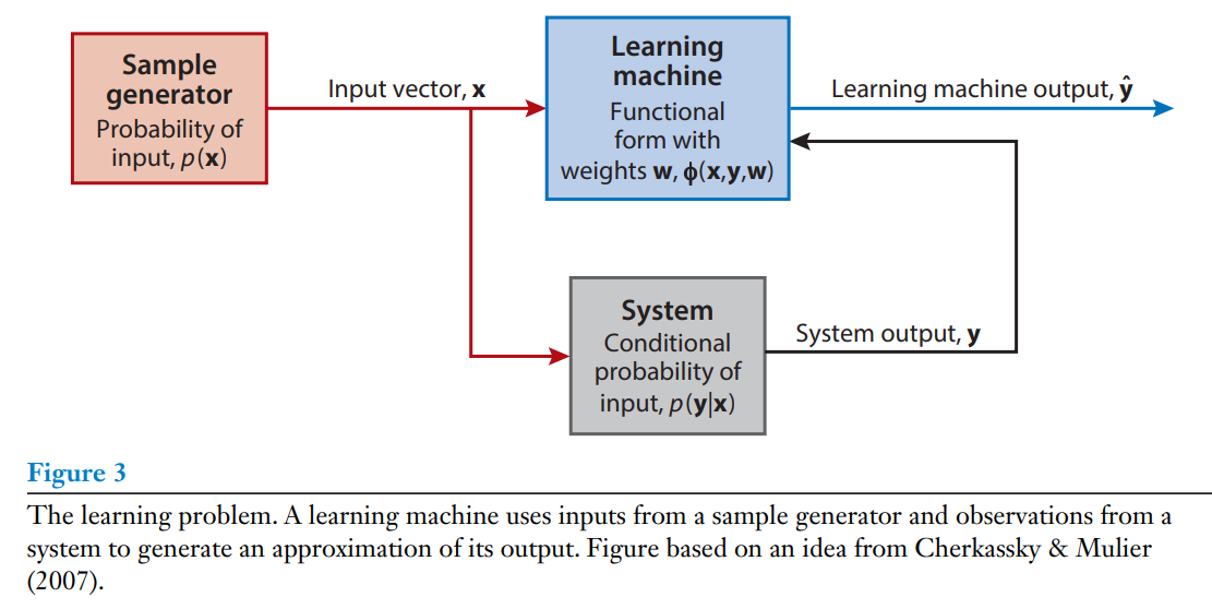
The learning problem can be formulated as the process of estimating associations between inputs, outputs, and parameters of a system using a limited number of observations (Cherkassky & Mulier 2007). We distinguish between a generator of samples, the system in question, and an LM, as in Figure 3. We emphasize that the approzimations by LMs are fundamentally stochastic, and their learning process can be summarized as the mininization of a risk functional:

$$R(\mathbf{w})=\int L[\mathbf{y}\mathbf{,}\mathbf{\Phi }\mathbf{(}\mathbf{x}\mathbf{,}\mathbf{y}\mathbf{,}\mathbf{w}\mathbf{)}\mathbf{]}\mathit{p}\mathbf{(}\mathbf{x}\mathbf{,}\mathbf{y}\mathbf{)}\mathrm{d}\mathbf{x}\mathrm{d}\mathbf{y},$$

where the data $\mathbf{x}$ (inputs) and  $\mathbf{y}$  (outputs) are samples from a probability distribution $ \mathit{p} $ , $ \mathbf{ \Phi(x,y,w)} $ defines the structure and $\mathbf{ w} $ the parameters of the LM, and the loss function $ L $ balances the various learning objectives (e.g. accuracy, simplicity smoothness, etc.). We emphasize that the risk functional is weighted by a probability distribution $ \mathit{p}(\mathbf{x,y}) $ that also constrains the predictive capabilities of the LM. The variout types of learning algorithms can be grouped into three major categories: superviesd, unsupervised, and semisupervised, as in Figure 1. These distinctions signify the degree to which external supervisory information from an expert is available to the LM. 

학습 문제는 제한된 수의 관측을 통한 데이터를 사용해 시스템의 입력과 출력, 그리고 매개편수 간의 연관성을 추정하는 과정으로 정의될 수 있다. Figure3에서 보이는 것처럼 학습 과정은 샘플 생성기와 문제를 푸는 시스템, 그리고 LM으로 구분되는 것을 알 수 있다. 여기서 강조할 점은 LM의 예측은 근본적으로 확률적이고 학습 방식은 다음과 같은 위험 함수(risk functional)를 최소화하는 것으로 나타낼 수 있다.

$$R(\mathbf{w})=\int L[\mathbf{y}\mathbf{,}\mathbf{\Phi }\mathbf{(}\mathbf{x}\mathbf{,}\mathbf{y}\mathbf{,}\mathbf{w}\mathbf{)}\mathbf{]}\mathit{p}\mathbf{(}\mathbf{x}\mathbf{,}\mathbf{y}\mathbf{)}\mathrm{d}\mathbf{x}\mathrm{d}\mathbf{y},$$

(Equation 1)

• $\mathbf{x}$(입력) 데이터와 $\mathbf{y}$ (출력) 데이터는 확률성 분포인 $\mathit{p}에서 추출된 샘플이고,
• $\mathbf{\Phi(x,y,w)}$ 는 학습머신의 구조를 정의하고,
• $\mathbf{w}$는 LM의 매개변수를,
• 그리고 손실함수 $L$ 은 정확성, 단순성, 부드러움 등의 다양한 학습 목포 간의 균형을 조정한다.

위험 함수는 $\mathit{p}(\mathbf{x,y})$ 에 의해 가중치가 부여되고, 이는 LM의 예측 능력을 제한하는 중요한 요소이다. 학습 알고리즘은 Figure 1에서 보았던 것처럼 지도, 비지도, 준지도 학습인 세 개로 크게 분류할 수 있는데, 이러한 분류는 LM이 전문가로부터 외부 감독 정보를 어느 정도 제공하느냐에 따라 구분되어진다.  

 

 

2.1 지도 학습

Supervised learning implies the availability of corrective information to the LM. In its simplest and most common form, this implies labeled training data, with labels corresponding to the output of the LM. Minimizatinon of the cost function, which depends on the training data, will determine the unknown parameters of the LM. In this context, supervised learining dates back to the regression and interpolation methids preposed centuries ago by Gauss (Meijering 2002). A commonly employed loss function is:

$$\mathit{L}[\mathbf{y}\mathbf{,}\mathbf{\Phi }\mathbf{(}\mathbf{x}\mathbf{,}\mathbf{y}\mathbf{,}\mathbf{w}\mathbf{)}\mathbf{]}\mathbf{=}\mathbf{|}\mathbf{|}\mathbf{y}\mathbf{-}\varphi \varphi \mathbf{(}\mathbf{x}\mathbf{,}\mathbf{y}\mathbf{,}\mathbf{w})|{|}^2$$

Alternative loss function may reflect different constraints on the LM such as sparsity (Hastie et al. 2009, Brunton & Kutz 2019). The choice of the approximation function reglects prior knowledge about the data, and the choice between linear and nonlinear methods directly bears on the computational cost associated with the learning methods. 

지도 학습은 LM에게 교정 정보를 제공할  수 있다는것을 의미한다. 가장 단순하고 일반적인 형태로는 라벨링된 훈현 데이터가 있을 것이며, 여기서 LM은 출력값으로 라벨을 뱉어낸다. 지도 학습의 목포는 학습 데이터에 의해 결정되는 비용 합수를 최소화해 LM의 미지의 매개변수를 결정하는 것이다.이런 식으로 보자면 지도 학습의 개념 수세기 전 가우스가 제안한 회귀(regression)와 보간 방법에까지 거슬러 올라갈 수 있다. 지도 학습에서 가장 보편적으로 사용되는 손실 함수는 다음과 같다:

$$\mathit{L}[\mathbf{y}\mathbf{,}\mathbf{\Phi }\mathbf{(}\mathbf{x}\mathbf{,}\mathbf{y}\mathbf{,}\mathbf{w}\mathbf{)}\mathbf{]}\mathbf{=}\mathbf{|}\mathbf{|}\mathbf{y}\mathbf{-}\varphi \mathbf{(}\mathbf{x}\mathbf{,}\mathbf{y}\mathbf{,}\mathbf{w})|{|}^2$$

(Equation 2)

대체 손실 함수는 희소성(sparsity)과 같은 다양한 제약 조건을 반영할 수 있다. 근사값을 측정하는 함수는 데이터에 대한 사전 지식을 반영하고, 이는 학습 방법과 모델의 효율성에 직접적으로 영향을 미치는 선형과 비선형 방식을 정하는 것에도 큰 영향을 미친다.

2.1.1 뉴럴 네트워크 (NN)

NNs are auguably the most well-known methods in supervised learning. They are fundamental nonlinear function approximators, and in recent years several efforts have been dedicated to understanding thier effectiveness. The universal approximation theorem (Hornik et al. 1989) states that any function may be approximated by a sufficiently large and deep network. Recent work has shown that sparsely connected, deep NNs are information theoretic-optiimal nonlinear approximators for a wide range of functions and systems (Bölcskeiet al. 2019).

NN은 지도 학습에서 가장 잘 알려진 방식일 것이다. NN은 기본적으로 비선형 함수의 근사 도구이며, 최근 이의 효용성을 이해하기 위한 다양한 연구가 진행되어 왔다. 보편 근사 정리(Universal Approximation Theorem)는 어떠한 예측 방식도 크고 깊은 네트워크를 이용하면 예측이 가능하다고 명시한다. 최근의 연구는 띄엄띄엄 연결돼있는(sparse connections) 깊은 신경망이 다양한 함수와 시스템에 대해 정보 이론적으로 최적의 비선형적 예측방법이라 나타내고 있다. 

The power and flexibility of NNs emanate from their modular structure based on the neuron as a central building element, a caricature of neurons on the human brain. Each neuron receives an input process it through an activation function, and produces an output. Multiple neurons can be combined into different structures that reflect knowledge about the problem and the type of data. Feedforward networks are among the most common structures, and they are composed of layers of neurons, where a weighted output form one layer is the input to the next layer. NN architectures have an input layer that receives the data and an output layer that produces a prediction. Nonlinear optimization methods, such as backpropagation (Rumelhart et al. 1986), are used to identify the network weights to minimize the error between the prediction and labeled training data. Deep NNs involve multiple layers and various types of nonlinear activation functions. When the activation functions are expressed in terms of convolutional kernels, a powerful class of networks emerges, namely convolutional neural networks (CNNs), with great success in image and pattern recognition (Krixhevsky et al. 2012, Goodfellow et al. 2016), Grossberg et al. 1988). 

신경망(NN)의 강력함과 유연성은 그들의 인간 두뇌의 뉴런을 본따 만든 모듈적 구조에서 온다. 각각의 뉴런은 입력을 받은것을 활성 함수를 통해 처리한 후 출력을 생성한다. 여러 개의 뉴런들을 결합하면 문제와 데이터 유형에 대한 지식을 반영하는 다양한 구조를 만들 수 있다. 순방향 신경망(Feedfoward network)은 가장 일반적인 구조 중 하나로, 이것은 여러 개의 뉴런으로 구성되어 있고 한 층의 출력이 다음 층의 입력이 된다. 신경망의 구조는 데이터를 받는 입력층과 예측값을 내보내는 출력층으로 이루어져 있다. 예측값과 라벨링된 학습 데이터 간의 오차를 최소화하기 위해 역전파(backpropagation)와 같은 비선형 최적화 방법이 사용되어 네트워크의 가중치를 학습한다. 신경망은 여러 개의 계층과 다양한 유형의 비선형 활성 함수가 사용된다. 특히, 활성화 함수가 합성곱 커널(convolutional kernels)의 형태로 표현될 때, 합성곱 신경망(CNN)이라고 하는 강력한 연결이 일어난다. CNN은 이미지나 패턴 인식에 큰 성공을 이루었다.  

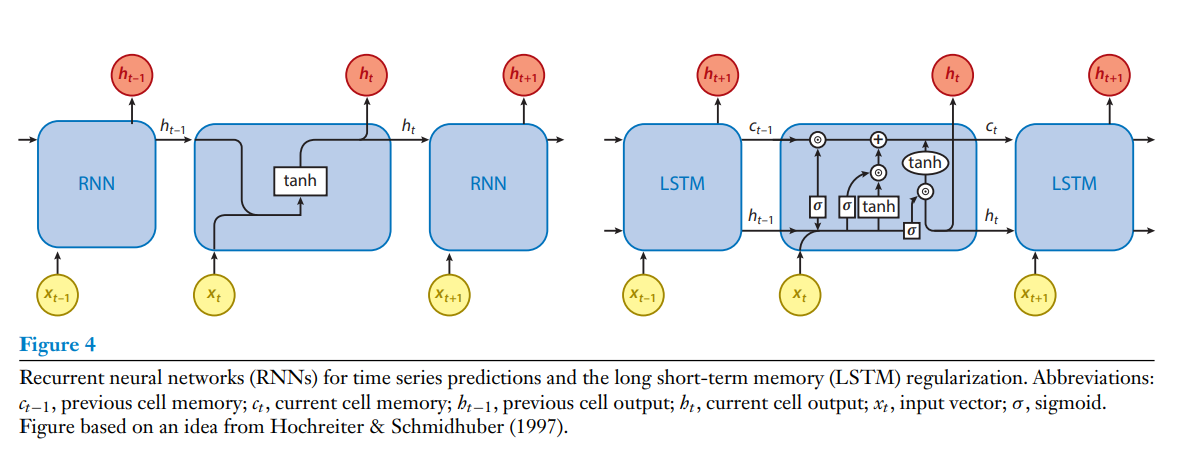
Recurrent neural networks (RNNs), depicted in Figure 4, are of particular interest to fluid mechanics. They operate on sequences of data (e.g., images from a video, time series, etc,), and thir weights are obtained by backpropagation through time. RNNs have been quite successfull for natural language processing and speech recognition. Their architecture takes into accout the inherent order of the data, thus augmenting some of the pioneering applications of classical NNs on signal processing (Rico-Marinez et al. 1992). However, their effectiveness has been hindered by diminishing or exploding gradients that emerge during their training. The renewed interest in RNNs is largely attributed to the development of the long short-term memory (LSTM) (Hochreiter & Schmidhuber 1997) algorithms that deploy cell states and gating mechanisms to store and forget information about past inputs, thus alleviating the problems with gradients and the transmission of lon-term information from which standard RNNs suffer. An extended architecture called the multidimensional LSTM network (Graves et al. 2007) was proposed to efficiently handle high-dimensional spatiotemporal data. Several potent alternatives to RNNs have appeared over the years; the echo state network has been used with success in predicting the output of several dynamical systems (Pathak et al. 2018).

Figure 4에 나타난 순환 신경망(RNN)은 특히 유체 역학에서 주목받는 구조로, 영상 이미지나 시계열 데이터 등의 연속적인 데이터에 활용되고 시간에 따른 역전파를 통해 가중치가 결정된다. RNN은 자연어 처리나 음석 인식에서 꽤 큰 성공을 이루었으며, 데이터의 고유한 순서를 고려한 구조이기 때문에 기존의 신명망에서 신호처리법을 응용해 보완하였다. 하지만, RNN은 효과성은 학습 과정에서 발생하는 기울기 소실(diminishing gradient) 또는 기울기 폭발(exploding gradient) 문제로 제한되었다. RNN이 새롭게 부각된 이유는 장단기 메모리(Long Short-Term Memory, LSTM) 알고리즘의 개발 덕분이다. RSTM 알고리즘은 셀의 상태와 게이팅 메커니즘(gating mechanism)을 사용해 이전의 입력 정보를 저장하고 삭제할 수 있이며, 이를통해 기존의 RNN이 겪고있던 기울기 문제나 장기 정보의 전달에 대한 한계를 극복하게 된다. 또한, 고차원의 시공간 데이터를 효율적으로 수행할 수 있는 다차원 LSTM 네트워크(multidimensional LSTM network) 구조가 제안되기도 하였다. RNN의 대안으로 에코 상태 네트워크(Echo State Network)와 같은 여러 동적 시스템을 성공적으로 예측하는것이 가능한 다른 모델들 등장하기도 하였다. 

2.1.2. 분류: 벡터 머신과 random forest 보조

Classification is a supervised learning tast that can determine the label or category of a set of measurements from a priori labeled training data. It is perhaps the oldest method for learning, starting with the perceptron (Rosenblatt 1958), which could classify between two types of linearly seperable data. Two fundamental classification algorithms are support vector machines (SVMs) (Schölkopf & Smola 2002) and random forest (Breiman 2001), which have been widely adopted in industry. The problem can be specified by the following loss functional, which is expressed here for two classes:

$$L[\mathbf{y}\mathbf{,}\mathbf{\Phi }\mathbf{(}\mathbf{x}\mathbf{,}\mathbf{y}\mathbf{,}\mathbf{w}\mathbf{)}]=\{\begin{array}{c}\text{0, if }\mathbf{y}\mathbf{=}\mathbf{\Phi }\mathbf{(}\mathbf{x}\mathbf{,}\mathbf{y}\mathbf{,}\mathbf{w}\mathbf{)},\\ \text{1, if }\mathbf{y}\ne \mathbf{\Phi }\mathbf{(}\mathbf{x}\mathbf{,}\mathbf{y}\mathbf{,}\mathbf{w}\mathbf{)}.\end{array}$$

The output of the LM is an indicator of the class to which the data belong. The rist functional quantifies the probability of misclassification, and the task is to minimize the risk based on the training data by suitable choice of $\mathbf{\Phi(x, y, w)}$. Random forests are based on an ensemple of decision trees that hierarchically split the data using simple conditional statements; these decisions are interpretable and fast to evaluate at scale. In the context of classification, an SVM maps the data into a high-dimensional feature space on which a linear classification is possible. 

분류(Classification)는 지도 학습의 한 형태로, 사전에 라벨링된 훈련 데이터를 바탕으로 측정값을 정할  집합에서 라벨이나 카테고리를 결정하는 작업이다. 이는 가장 오래된 학습 방법 중 하나로, 1958년 Rosenblat이 시작한 선형적으로 구분이 가능한 두 가지 데이터를 분류하는 퍼셉트론에서 시작하였. 산업계에서 널리 채택된 두 가지 기본적인 분류 알고리즘은 서포트 벡터 머신(SVM)과 랜덤 포레스트(random forest) 방법이다. 이 문제는 아래에 보이는 두개의 클래스로 손실 함수로 특정지을 수 있다:

$$L[\mathbf{y}\mathbf{,}\mathbf{\Phi }\mathbf{(}\mathbf{x}\mathbf{,}\mathbf{y}\mathbf{,}\mathbf{w}\mathbf{)}]=\{\begin{array}{c}\text{0, if }\mathbf{y}\mathbf{=}\mathbf{\Phi }\mathbf{(}\mathbf{x}\mathbf{,}\mathbf{y}\mathbf{,}\mathbf{w}\mathbf{)},\\ \text{1, if }\mathbf{y}\ne \mathbf{\Phi }\mathbf{(}\mathbf{x}\mathbf{,}\mathbf{y}\mathbf{,}\mathbf{w}\mathbf{)}.\end{array}$$

(Equation 3)

LM의 출력값은 해당 데이터가 어디에 분류되는지를 나타낸다. 위험 함수는 잘못 분류되었을 확률을 계산하고, 훈련 데이터를 바탕으로  $\mathbf{\Phi(x, y, w)}$를 적절히 선택해 손실을 최소화하는 것이 목표다. 랜덤 포레스트는 간단한 조건문으로 데이터를 계층적으 분할하는 의사결정 트리(Decision Tree)의 합주(ensemble)에 기반한다. 이 결정은 해석이 가능하고 대규모 데이터도 빠르게 계산할 수 있다. 분류의 개념으로 봤을 때, SVM은 데이터를 고차원적인 공으로 재배열해 선형 분류가 가능하게 한다. 

2.2 비지도 학습

This learning task implies the extraction of features from the data by specifying certain global criteria, without the need for supervision of a ground-truth. The types of problems involved here include dimensionnality reduction, quantization, and clustering. 

비지도 학습법은 감독이나 검증 자료 없이 전체적인 기준을 특정지어 데이터의 특을 빼낸다. 이 학습 방식에서 다루는 문제 유형에는 차원의 축소(dimensional reduction)나  양자화(quantization), 그리고 군집화(clustering)가 포함된다. 

2.2.1 차원 축소 I:  적절 직교 분해(POD, Proper Orthogonal Decomposition), 주성분 분석(PCA, Principal Conponent Analysus), 및 오토인코더(Autoencoder)

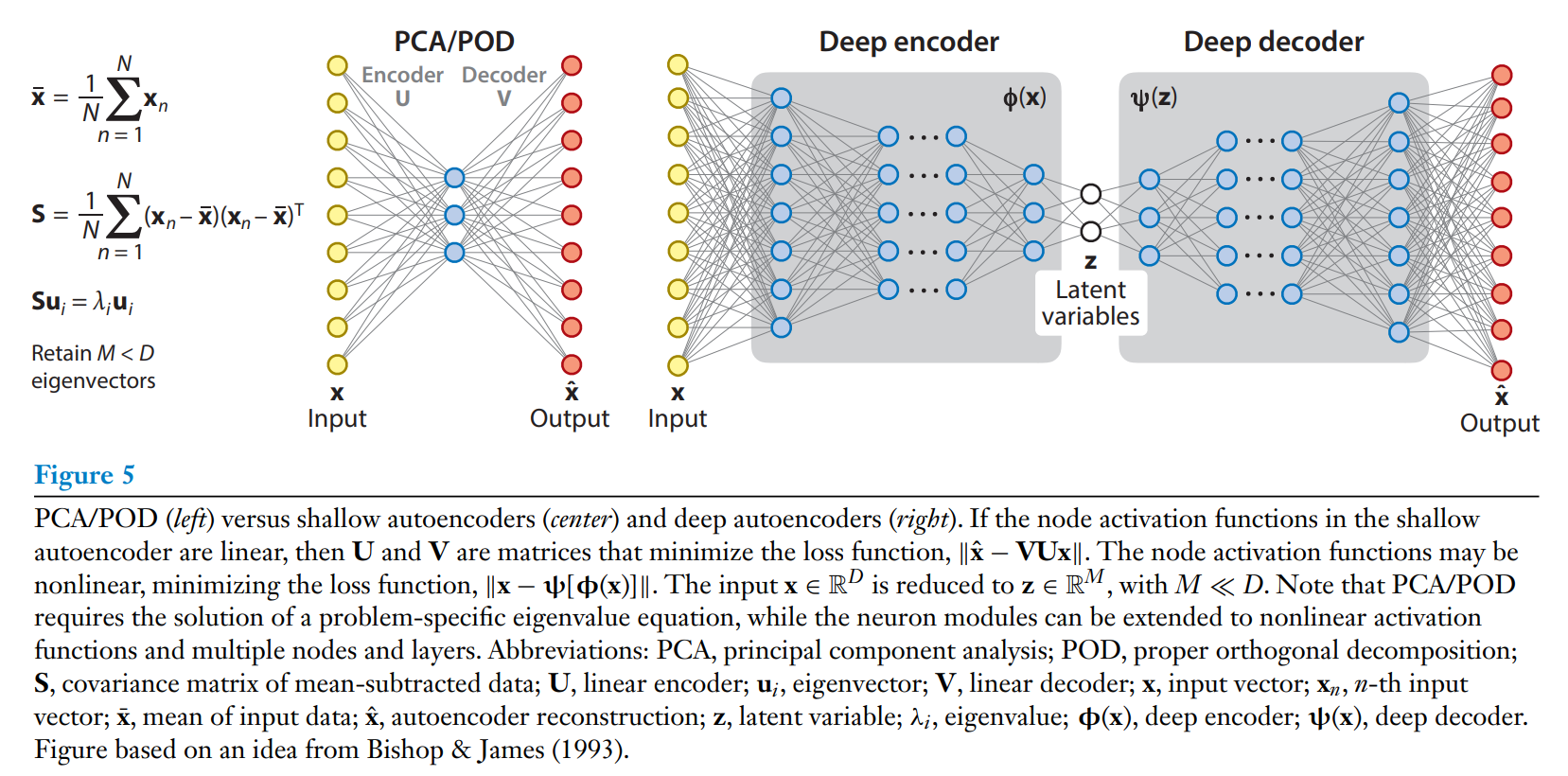
 The extraction of flow features from experimental data and large-scale simulations is a cornerstone of flow modeling. Moreover, identigying lower-dimentsioal representatins for high-dimensional data can be used as preprocessing for all tasks in supervised learning algorithms. Dimensionality reduction can also be viewed as an information-filtering bottleneck where the data are processed through a lower-dimentsional representation before being mapped back to the ambient dimension. The classical POD algorithm belongs to this category is learning and is discussed more in Section 3. The POD, or linear principal componenet analysis(PCA) as it is more widely known, can be formulated as a two-layer NN (an autoencoder) with a linear activation function for its linearly weighted input, which can be trained by stochastic gradient descent (see Figure5). This formulation is an algorythmic alternative to linear eigenvalue/eigenvector problems in terms of NNs, and it offers a direct route to the nonlinear regime and deep learning by adding more layers and a nonlinear activation function on the network. Unsupervised learning algorithms have seen limited use in the fluid mechanics community, and we believe that they deserve further exploration. Inrecent years, the ML community has developed numerous autoencoders that, when properly matched with the possible features of the flow field, can lead to significant insight for reduced-order modeling of stationary and time-dependent data. 

유체 모델링의 핵심 요소는 실험 데이터와 대규모 시뮬레이션에서 유체의 특징을 뽑아내는 것이다. 또한, 지도 학습 알고리즘을 위해 고차원 데이터를 저차원으로 표현함으로 전처리 과정으로 활용할 수 있다. 차원의 축소라 함은, 데이터를 저차원으로 표현한 후 다시 원래 차원으로 매핑하는 정보 필터링의 병목 현상으로도 볼 수 있다. 전통적인 POD 알고리즘이 이러한 학습 범주에 속하는데, 이는 3장에서 더 자세히 논의될 것이다. POD는 선형 주성분 분석(PCA)으로도 널리 알려져 있는데, 이것은 .확률적 경사 하강법(stochastic gradient descent)으로 학습된 선형 가중이 매겨진 입력값의 2층짜리 신경망(오토 인코더)으로 구성될 수 있다. 이러한 구성은 선형 고유값이나 고유 벡터 문제를 신경망 관점에서 해결하는 알고리즘적 대안으로, 네트워크에 더 많은 층과 비선형적 활성 함수를 추가함으로서 비선형적인 영역과 딥러닝에 직접적으로 확정할 수 있는 경로를 제공한다. 비지도 학습은 유체 역학 분야에서는 제한적으로만 사용되고 있는데, 이것은 미래에 더한 연구가 필요할 것이다. 최근 연구에서 ML 분야 다양한 오토 인코더를 개발했으며, 이러한 오토 인코더가 유동장의 몇몇 특징들과 적절히 맞아 떨어진다면, 정적이거나 시간에 의존된 데이터를 위한 저차원 모델링(reduced-order modeling)에 중요한 통찰을 제공할 수 있다. 

 

2.2.2. 차원 축소II: 이산 주곡선(DPC, Discrete Princial curves)와 자기 조직화 지도(SOM, Self-Organizing Maps)

The mapping between high-dimensional data and a low-dimensional representation can be structured through an explicit shaping of the lower-dimensional space, possibly reflecting and priori knowledge about this subspace. These techniques can be seen as extensions of the linear autoencoders, where the encoder and decoder can be nonlinear functions. This nonlinearity may, however, come at the expense of losing the inverse relationship between the encoder and decoder functions that is one of the strengths of linear PCA. Analternative is to define the decoder as an approximation of the inverse of the encoder, leading to the method of principal curves. Principal curves are structures on which the data are projected during the encoding step of the learning algorithm. In turn, the decoding step amounts to an approximation of the inverse of this mapping by adding, for example, some smoothing into the principal curves. An important version of this process is the self-organizing map (SOM) introduced by Grossberg(1976) and Kohonen (1995). In SOMs the projection subspace is described into a finite set of values with specified connectivity architecture and distance metrics. The encoder step amounts to identifying for each data point the closest node point in the SOM, and the decoder step is weighted regression estimate using, for example, kernel functions that take advantage of the specified distance metric between the map nodes.  This modifies the node centers, and the process can be iterated until the empirical risk of the autoencoder has been minimized. The SOM capabilities can be exemplified by comparing it to linear PCA for a two-dimensional set of point. The linear PCA will provide as an approximation the least squares straignt line between the points, whereas the SOM will map the points onto a curved line that better approximates the data. We note that SOMs can be extended to areas beyond floating point data, and they offer an interesting way for creating databases based on features of flow fields. 

고차원 데이터와 저차원 표현간의 매핑을 위해서는 저차원의 공간을 명시적으로 형성하는 방식으로 구성할 수 있으며, 이는 하위 공간에 대한 사전 지식을 바탕으로 반영할 수도 있다. 이러한 기법은 선형적 오토 인코더 기술의 확장이라고 생각하면 되는데, 여기에서 인코더와 디코더는 비선형적 함수로 정의될 수 있다. 하지만 이러한 비선형성은 선형 PCA의 강점 중 하나인 인코더와 디코더 함수 간의 역 관계를 사용하지 못하게 될 수 있다. 다른 방법으로는 디코더를 인코더의 역함수에 대한 근사치로 정의하는 것으로, 이는 주곡선(principal curves) 기법으로 이어진다. 주곡선이라 함은 학습 알고리즘의 인코딩 단계에서 투영된 데이터의 구조를 말한다. 이후, 디코딩 단계에서는 예를 들어 주곡선에 스무딩(smoothing)을 추가함으로서 해당 매핑의 역함수의 근사값을 얻는다. 이 단계의 중요한 버전 중 하나는 1976년 Grossberg와 1995년 Kohonen에 의해 소개된 자기 조직화 지도(SOM)가 있다. SOM에서 투영된 하위 공간이라 함은 특정한 연결된 구조이거나, 거리의 측정 기준이 지정된 유한한 값의 세트이다. 인코더 단계에서는 각각의 데이터 포인트에 대해 SOM으로 계산된 가장 가까운 노드 포인트를 식별한다. 그리고 디코더의 단계에서는 지정된 거리 기준을 활용한 커널 함수 등을 사용해여 가중 회귀의 추정(weighted regression extimate)을 수행한다. 이러한 방식으로 노드의 중심이 조정되고, 오토 인코더의 경험적 리스크(empirical risk)가 최소화되기 전까지 반복된다. SOM의 성능은 2차원 데이터 세트를 대상으로 선형 PCA와 그 값을 비교하며 확인할 수 있다. 선형 PCA는 데이터 포인트들 사이의 최소 제곱직선을 근사치로 나타낸다. 반면, SOM은 데이터 넘어 그 이상의 영역으로 확장될 수 있으며, 이것은 유동장의 특징에 기반된 데이터베이스를 생성하는 흥미로운 방법이 될 것이다. 

2.2.3. 군집화(clustering)와 벡터 양자화(vector quantization)

    Clustering is an unsupervised learning technique that identifies similar groups in the data. The most common algorithm is k-means clustering, which partitions data into k clusters; an observation belongs to the cluster with the nearest centroid, resulting in a partition of data space into Vorovoi cells. 

Vector quantizers identify representative points for data that can be partitioned into a predetermined number of clusters. These points can then be used instead of the full data set so that future samples can be approximated by them. The vector quantizer $\Phi(\mathbf{x,w})$ provides a mapping between the data $\mathbf{x}$ and the coordinates of the cluster centers. The loss function is usually the squared distortion of the data from the cluster centers, which must be minimized to identify the parameters of the quatizer,

$$L[\Phi(\mathbf{x,w})] = ||\mathbf{x-\Phi(x,w)}||^2$$

    We note that vector quantization is a data reduction method not necessarily employed for dimensionality reduction. In the latter, the learning problem seeks to identify low-dimensional features in high-demensional data, whereas quantization amounts to finding representative clusters of the data. Vector quantization must also be distinguished from clustering, as in the former the number of desired centers is determined a priori, whereas clustering aims to identify meaningful groupings in the data. When these groupings are represented by some prototypes, then clustering and quantization have strong similarities. 

    군집화(clustering)는 데이터를 유산한 특성을 가진 그룹으로 나누는 비지도 학습 기법이다. 가장 일반적인 알고리즘은 k-평균 군집화(k-means clustering)으로, 데이터를 k개의 군집들로 분류한다. 이 과정에서 데이터는 가장 가까운 중심점(centroid)을 가진 그룹에 속하게 되고, 이 데이터 공간은 Voronoi 셀을 이용해 분류한다. 

    벡터 양자화는 데이터를 사전에 정의된 수의 군집으로 나눌 수 있는 대표적인 점(representative points)들을 식별하는 과정이다. 이러한 점들은 이후에 전체 데이터 대신에 사용될 수 있고, 이를 통해 미래의 샘플 데이터의 유사값이 결정된다. 벡터 양자화 $\Phi(\mathbf{x,w})$는 데이터 $\mathbf{x}$와 군집의 중심의 죄표 간의 매핑을 제공한다. 이 과정에서 손실 함수는 군집의 중심으로부터 데이터의 왜곡의 제곱(squared distortion)을 최소화하는 데 기반하며, 이것은 매개변수의 양자를 식별하기 위해 다음의 수식으로 최소화된다:

$$L[\mathrm{\Phi }(\mathbf{x}\mathbf{,}\mathbf{w})]=||\mathbf{x}\mathbf{-}\mathbf{\Phi }\mathbf{(}\mathbf{x}\mathbf{,}\mathbf{w}\mathbf{)}|{|}^2$$

(Equation 4)

여기서 벡터 양자화란 데이터를 축소하기 위한 방법으로, 꼭 차원 축소에 사용되는 것은 아니다. 차원 축소에서는 고차원 데이터에서 저차원적 특징을 식별하는 문제를 다루는 반면, 양자화는 데이터를 대표하는 군집을 찾는 데 초점을 둔다. 벡터 양자화와 군집화 또한 서로 구분되는데, 벡터 양자화에서는 원하는 중심점의 개수를 미리 지정하는데 반해, 군집화는 데이터 내에서 의미가 있는 군집들을 식별해 나간다는 사실이 서로 다르다. 다만, 이러한 그룹이 표본으로 제시된다면, 군집화와 양자화는 강한 유사성을 가지게 된다.  

2.3. 준지도 학습

Semisupervised learning algorithms operate under partial supervision, either with limited labeled training data or with other corrective information from the environment. Two algorithms in this category are generative adversarial networks (GANs) and RL. In both cases, the LM is (self-)trained through a game-like process discussed below. 

준지도 학습은 부분적인 지도 아래 학습되는 알고리즘은데, 한정적으로 라벨링된 학습 데이터 이거나, 주위 환경에서 제공되는 다른 형태의 교정 정보를 기반으로 학습하는 것이다. 이 범주에 속하는 두 가지의 알고리즘은 생성적 적대 신경망(GAN, Generative Adversarial Networks)과 강화학습(RL, Reinforcement Learning)이다. 두 알고리즘 모두게임과 같은 과을 통해 (자기주도적으로) 학습을 진행하며, 이에 대한 자세한 내용은 아래에서 논의된다. 

2.3.1. 생성적 적대 신경망 (GAN, Generative Adversarial Networks)

GANs are learning algorithms that result in a generative model, i.e., a model that produces data according to a probability distribution that mimics that of the data used for its training. The LM is composed of two networks that compete with each other in a zero-sum game (Goodfellow et al. 2014). The generative network produces candidate data examples that are evaluated by the discriminative, or critic, network to optimize a certain task. The generative network's training objective is to synthesize novel examples of data to fool the discriminative network into misclassifying them as belonging to the true data distribution. The weights of these networks are obtained through a process, inspired by game theory, called adversarial learning. The final objective of the GAN training process is to identify the generative model that produces an output that reflects the underlying system. Labeled data are provided by the discriminator network, and the function to be minimized is the Kullback-Liebler divergence between the two distributions. In the ensuing game, the discriminator aims to maximize the probability of discriminating between true data and data produced by the generator, while the generator aims to minimize the same probability.  Because the generative and discriminative networks essentially train themselves, after initialization with labeled training data, this procedure is often called self-supervised. The self-training process adds to the appeal of GANs, but at the same time one must be cautious about whether an equilibrium will ever be reached in the above-mentioned game. As with other training algorithms, large amounts of data help the process, but at the moment, there is no guarantee of convergence. 

GAN은 학습된 데이터의 확률 분포를 모방하여 데이터를 출력하는 모델을 만드는 생성적 학습 알고리즘이다. GAN은 두 개의 네트워크로 구성되며, 이들은 제로섬 게임에서 서로 경쟁하도록 되어 있다. 생성 신경망(generator)은 데이터 예제를 생성하며, 판별 신경망(discriminator 또는 critic)는 생성된 데이터가 실제 데이터 분포에 속하는지를 판별한다. 생성 신경망의 목표는 판별 신경망을 교란시켜 생성된 데이터를 실제 데이터를 오분류하게 만드는 것이다. GAN의 학습 목표는 적대적 학습이라는 게임 이론에 영감을 받아 만들어졌다. GAN 학습법의 최종 목표는생성 신경망이 내제된 시스템의 실제 분포를 반영하는 데이터를 출력값으로 내놓는 모델을 만드는 것이다. 판별 신경망은 라벨링된 데이터를 기반으로 훈련되고, 최적화 함수는 두 분포 간의 Kullback-Liebler 발산을 최소화하는 것이다. 이어지는 게임에서, 판별 신경망은 실제의 데이터와 생성자에 의해 만들어지 데이터를 구분할 확률을 최대화하고, 생성 신경망은 동일한 확률을 최소화하는데 목표를 둔다. 생성자와 판별자는 결과적으로 그들 자신을 학습시키기 때문에, 라벨링 된 학습 데이터로 시작한 이후로의 진행 방식은 때로 자기 지도 학습(self-supervised learning)이라고 불린다. 자기 스스로 학습하는것은 GAN의 장점이지만, 위에 언급된 게임과 같은 균형 상태(equilibrium)를 얻는것을 조심해야 한다. 다른 알고리즘처럼, 데이터가 많을수로 학습에 도움이 되긴 하지만, 현재로서는 GAN이 반드시 수렴할 것이라는 보장은 없다. 

2.3.2. 강화 학습(RL)

RL is a mathematical framework for problem solving (Sutton & Barto 2018) that implies goal-directed interactions of an agent with its environment. In RL the agent has a reperttoire of actions and perceives states. Unlike in supervised learning, the agent does not have labeled information about the correct actions but instead learns form its own experiences in the form of rewards that may be infrequent and partial; thus, this is termed semisupervised learning. Moreover, the agent is concerned not only with uncovering patterns in its actions of in the environment but also with maximizing its long-term rewards. RL is closely linked to dynamic programming (Bellman 1952), as it also models interactions with the environment as a Markov decision process. Unlike dynamic programming, RL does not require a model of the dynamics, such as a Markov transition model, but proceeds by repeated interaction with the environment through trial and error. We believe that it is precisely this approximation that makes it highly suitable for complex problems in fluid dynamics. The two central elements of RL are the agent's policy, a mapping $a=\pi(s)$ between the state $s$ of the system and the optimal action $a$, and the value function $V(s)$ that represents the utility of reaching the state $s$ for maximizing the agent's long-term rewards. 

강화 학습은 문제 해결을 위한 수학적 프레임워크로, 에이전트와 환경 간의 목표 지향적인 상호작용을 포함하고 있다. 강화 학습에서 요원은 행동하는 레퍼토리를 가지고 있으며, 환경의 상태를 인식한다. 지도 학습과는 다르게, 에이전트는 올바른 행동이 무엇인지 적힌 정보를 제공받지 않는다. 대신에 보상을 받는 형태로 학습하며, 이 보상은 흔하게 제공되지 않을 수 있으며, 부분적일 수도 있다. 그러므로 이건 준지도 학습이라고 불린다. 요원은 행동을 통해 환경의 패턴을 알아내는것 뿐만 아니라 장기 보수를 최대화하는 데 초점을 둔다. 강화 학습은 1952년 Bellman이 제시한 동적 프로그래밍과 밀접한 관련이 있는데, 이 또한 환경과의 상호작용을 마르코프 의사 결정법에 의해 모델링한다. 동적 프로그래밍과는 달리, 강화 학습은 마르코프 전이 모델과 같은 동적 모델이 필요하지 않지만, 환경과 반복적으로 상호작용하며 시행착오를 통해 학습한다. 바로 이러한 점이 복잡한 유체역학의 문제에 적합한 이유가 될 수 있다. 강화 학습의 핵심 요소는 요원의 정책이라고 할 수 있는데, 이는 시스템의 상태 $s$와 최적의 행동 $a$ 사이의 매핑 $a=\pi(s)$을 정의한다. 그리고 상태 $s$에 도달하는 것이 에이전트에게 주는 장기적인 보상을 극대화하는 데 얼마나 유용한지를 나타내는데 가치 함수 $V(s)$를 사용한다. 

Games are one of the key applications of RL that exemplify its strengths and limitations. One of the early success of RL is the backgammon learner of Tesauro (1992). The program started out from scratch as a novice player, trained by playing a couple of million times against itself, won the computer backgammon olympiad, and eventually became comparable to the three best human players in the world. In recent years, advances in high-performance computing and deep NN architectures have produces agents that are capable of performing at or above human performance at video games and strategy games nuch more complicated that backgammon, such as Go (Mnih et al. 2015) and the AI gym (Mnih et al. 2015, Silver et al. 2016). Its important to emphasize that RL requires significant computational resources due to the large numbers of episides required to properly account for the interaction of the agent and the environment. The cost may be trivial for games, but it may be prohibitive in experiments and flow simulations, a situation that is rapidly changing (Verma et al. 2018). 

게임은 강화 학습의 강점과 한계를 잘 보여주는 대표적인 응용 사례이다. 강화 학습의 초기 성공 성공 사례 중 하나는 1992년 행해진 테사우로의 백게먼(일종의 주사위 보드게) 학습이었다. 이 프로그램은 아무것도 모르는 초보자로 시작해 자기자신을 대상으로 수백만번의 플레이를 한 뒤, 컴퓨터 백게먼 올림피어드에서 우승하였고, 결국 세계에서 가장 뛰어난 세 명의 인간 선수 세 명과 비견될 정도의 실력을 갖추기도 하였다. 최근에 와서는 컴퓨터의 눈부신 발전과 신겨망 구조의 발전으로, 강화 학습 에이전트는 주사위게임보다 더 복잡한, 예를 들어 바둑과 같은, 비디오 게임이라던지 전략 게임에서 인간과 비슷하거나 더 뛰어난 성능을 보이기도 하였다. 이러한 발전은 강화 학습을 의한 AI 시뮬레이션 플랫폼은 AI Gym에서도 확인될 수 있다. 여기서 잊지 말아야 할 것은, 강화 학습은 에이전트와 환경 간의 수많은 에피소드를 필요로 하기 때문에 막대한 계산 자원의 필요하다는 것이다. 게임과 같은 가상세계에서 이러한 비용은 사소하겠지만, 실험적 환경이나 실험이나 유동 시뮬레이션에서는 엄두도 못할 계산 비용이 나올 수 있다. 하지만 이러한 비용 문제는 빠르게 변하고 있고, 점점 더 효율적인 학습 환경과 기술이 개발되고 있다.  

A core remaining challenge for RL is the long-term credit assignment (LTCA) problem, especially when rewards are sparse or very delayed in time (for example, consider the case of a perching bird or robot). LTCA implies inference, from a long sequece of states and actions, of casual relations between individual decisions and rewards. Several efforts address these issues by augmenting the original sparsely rewarded objective with densely rewarded subgoals (Schaul et al. 2015). A related issue is the proper accounting of past experience by the agent as it actively forms a new policy (Novati et al. 2019). 

강화 학습에 남아있는 핵심 과제 중 하나는 장기 신용 할당(LTCA, long-term credit assignment)이다. 특히 보상이 드물거나 매우 지연될 경우, 예를 들면 새나 로봇이 착륙하는 상황, 에서 이러한 문제가 두드러진다. LTCA는 긴 상태와 행동 시퀀스에서 각각의 결정과 보상 간의 인과 관계를 추론하는 것을 의미한다. 이문제를 해결하기 위해 여러 연구가 진행되고 있으며, 보상이 적은 목표를 보완하기 위해 조밀하게 보상되는 하위 목표를 추가하는 방식이 제안되기도 했다. 또한 관련된 문제로는 에이전트가 새로운 정책을 형성하면서 과거의 경험을 반영하는 것이 있을 것이다.

2.4. 확률적 최적화: 학습 알고리즘의 관점으로

Optimization is an inherent part of learning, as a rist functional is minimized in order to identify the parameters of the LM. There is, however, one more link that we wish to highlight in this review: that optimization (and search) algorithms can be cast in the context of learning algorithms and more specifically as the process of learning a probability distribution that contains the design points that maximize a certain objective. This connection was pioneered by Rechenberg (1973) and Schwefel (1977), who introduced evolution strategies (ES) and adapted the variance of their search space based on the success rate of their experiments. This process is also reminiscent of the operations of selection and mutation that are key ingredients of genetic algorithms (GAs) (Holland 1975) and genetic programming (Koza 1992). ES and GAs can be considered as hybrids between gradient search strategies, which may effectively march downhill toward a minimum, and Latic hypercube or Monte Carlo sampling methods, which maximally explore the search space. Genetic programming was developed in the late 1980s by J.R. Koza, a PhD student of John Holland. Genetic programming generailized parameter optimization to function optimization to function optimization, initially coded as a tree of operations (Koza 1992). A critical aspect of these algorithms is that they rely on an iterative construction of the probability distribution, based on data values of the objective function. This iterative construction can be lengthy and practically impossible for problems with expensive objective function evalutions.  

최적화는 학습의 본질적인 부분으로, 위험 함수(risk function)를 최소화하여 학습 모델(LM)의 매개변수들의 알아보기 위한 과정을 포함하고 있다. 그러나 이 리뷰에서 강조하고자 하는 또 다른 연결점은 최적화와 탐색(search) 알고리즘이 학습 알고리즘의 학습 알고리즘의 맥락에서 해석될 수 있다는 점이다. 구체적으로 말하자면, 이 알고리즘들은 특정한 목표을 극대화하는 설계 지점을 포함하는 확률 분포를 학습하는 과정으로 학습알고리즘에 적용시킬 수 있다는 것이다. 이러한 연결은 1973년 Rechenberg와 1977년 Schwefel에 의해 개척되었으며, 이들은 진화 전략(evolution strategy, ES)을 도입해 실험의 성공률에 기반해 탐색 공간의 분산을 조정하였다. 이런 진행방향은 Holland(1975)의 유전적 알고리즘(genetic algorithms, GAs) 및 유전 프로그래밍(Genetic Programming)에서의 선택된 몇몇만이 진화의 주요 재료라는 연구결과와 비슷하다. ES와 GA는 기울기 탐색 전략(gradient search strategies)과 유사하게 작동하며, 이는 최소화를 향해 점점 진행되는 라틴 하이퍼큐브(Latin Hypercube)나 몬테 카를로(Monte Carlo) 샘플링 방법처럼 탐색 공간을 최대한 탐구하기도 한다. 유전 프로그래밍은 1980년대 후반, John Holland의 박사과정 학생인 J.R. Koza에 의해 개발되었다. 유전 프로그래밍은 매개변수의 최적화를 함수의 최적화로 확장하였으며, 초기에는 트리 형태의 연 방식(tree of operations)으로 최적화 되도록 프로그로밍 되어졌다. 이러한 알고리즘의 핵심 측면은 목표 함수의 데이터 값에 기반해 확률 분포를 반복적으로 구성하는 점이다. 그러나 이런 반복적인 구성은 시간이 오래 걸리 수 있으며, 목표 함수 평가 비용이 높은 문제들에서는 실질적으로 계산이 불가능할 수 있다.

Over the past 20 years, ES and GAs have begun to converge into estimation of distribution algorithms (EDAs). The covariance matrix adaptation ES (CMA-ES) algorithm (Ostermeier et al. 1994, Hansen et al. 2003) is a prominent example of ES using an adaptive estimation of the covariance matrix of a Gaussian probability distribution to guide the search for optimal parameters. This covariance matrix is adapted iteratively using the best points in each iteration. The CMA-ES is closely related to several other algorithms, such as mixed Bayesian optimization algorithms (Pelikan et al. 2004), and the reader is referred to Kern et al. (2004) for a comparative review. In recent years, this line of work has evolved into the more generalized information-geometric optimization (IGO) framework (Ollivier et al. 2017). IGO algorithms allow for families of probability distributions whose parameters are learned during the optimization process and maintain the cost function invariance as a major design principle. The resulting algorithm makes no assumption on the objective function to be optimized, and its flow is equivalent to a stochatic gradient descent. These techniques have proven to be effective on several simplified benchmark problems; however, their scaling remains unclear, and there are few gurantees for convergence in cost function landscapes such as those encountered in complex fluid dynamics problems. We note also that there is an interest in deploying these optimization methods to minimize the cost functions often associated with classical ML tasks (Salimans et al. 2017). 

지난 20년 동안 ES와 GA는 분포 알고리즘(Estimation of Distribution Algorithms, EDAs)으로 수렴하기 시작했다. 공분산 행렬 적응 진화 전략(Covariance Matrix Adaptation ES, CMA-ES) 알고리즘은 이에 대한 대표적인 사례로, 최적 매개변수를 탐색하기 위해 가우시안 확률 분포의 공분산 행렬을 적응적으로 추정한다. 이러한 공분산 행렬은 각각의 반복 단계에서 가장 우수한 점들을 사용해 반복적으로 조정된다. CMA-ES는 혼합 베이지안 최적화 알고리즘(Mixed Bayesian Optimization Algoritms)과 밀접한 관련이 있으면, 이는 Kern et al.(2004)의 비교 리뷰에서 더 자세히 알아볼 수 있다. 최근에 와서 이러한 연구는 정보 기하학 최적화 (IGO, Information-Geometric Optimization)프레임워크로 발전하였다. IGO 알고리즘은 최적화 진행 도중에 매개변수가 학습되는 확률 분포의 계열을 허용하며, 비용 함수 불변성(cost function invariance)을 주요 설계 원칙으로 유지한다. 결과적으로 생성된 알고리즘은 최적화할 비용 함수에 대한 가정을 하지 않으며, 그 흐름은 확률적 경사 하강법과 동등하다. 이러한 기술들은 단순화된 벤치마크 문제에는 효과적인 걸로 입증되었으나, 스케일링 문제는 아직 명확하지 않으며, 복잡한 유체 역학문제와 같은 비용 함수 지형에서의 수렴 보장은 거의 없다. 또한, 이러한 최적화 방법을 클래식 ML 작업과 관련된 비용 함수를 최소화하는데 사용하는 것에 대한 관심도 증가하고 있음을 Salimans et al.(2017)의 연구에서 확인할 수 있다.

2.5. 이 리뷰에서 다루지 않는 중요한 주제: 베이시안 추론과 가우시안 프로세스

There are several learning algorithms that this review does not address but that demand particular attention from the fluid mechanics community. First and foremost, we wish to mention Bayesian inference, which aims to inform the model structure and its parameters from data in a probabilistic framework. Bayesian inference is fundamental for uncertainty quantification, and it is also fundamentally a learning method, as data are used to adapt the models. In fact, the alternative view is also possible, where every ML framework can be cast in a Bayesian framework (Barber 2012, Teodoridis 2015). The optimization algorithms outlined in this review provide a direct link. Whereas optimization algorithms aim to provide the best parameters of a model for given data in a stochastic manner, Bayesian inference aims to provide the full probability distribution. It may be argued that Bayesian inference may be even more powerful than ML, as it provides probability distributions for all parameters, leading to robust predictions, rather than single values, as is usually the case with classical ML algorithms. However, a key drawback for bayesian inference is its computational cost, as it involves sampling and integration in high-dimensional spaces, which can be prohibitive for expensive function evaluations (e.g., wind tunnel experiments or large-scale direct numerical simulation). Along the same lines, one must mention Gaussian processes (GPs), which resemble kernel-based methods for regression. However, GPs develop these kerenels adaptively based on the available data. They also provide probability distributions for the respective model parameters. GPs have been used extensively in problems related to time-dependent problems, and they may be considered competitors, albeit more costly, to RNNs. Finally, we note the use of GPs as surrogates for expensive cost functions in optimization problems using ES and GAs. 

이 리뷰에서는 다루지 않지만 유체역학 분야에서 특별한 관심을 필요로 하는 학습 알고리즘이 있다. 그중 첫번째로 베이시안 추론(Bayesian inference)이 있는데, 이는 확률론적 프레임워크 안에서 데이터로부터 모델 구조와 매개변수를 도출하는 것이다. 베이시안 추론은 불확실성 정량화(uncertainty quantification)의 근본적인 도구이자, 이것 또한 데이터가 모델을 적응시키기 위한 학습 방법이다. 사실, 이를 반대로 볼 수도 있닌데, 모든 ML 프레임워크가 베이시안 프레임워크 내에서 표현될 수 있다는 것이다(Barber, 2012; Theodoridis, 2015). 이 리뷰에서 설명된 최적화 알고리즘들은 이를 직접적으로 연결한다. 최적화 알고리즘이 주어진 데이터 대한 모델의 최적 매개변수를 제공하지만, 베이시안 추론은 전체 확률 분포를 제공한다. 베이시안 추론은 모든 매개변수에대한 확률 분포를 제공하므로, 단일 값만 예측하는 전통적인 ML 보다 더 견고한 예측(robust predictions)이 가능한 강력한도구일 수 있다. 그러나 베이지안 추론의 주요 단점은 계산 비용인데, 고차원 공간에서 샘플링과 적분을 수행해야 하기 때문에 풍동 실험이라거나 큰 스케일의 직접 수치 시뮬레이션과 같은 비싼 함수 계산에서는 제한될 수 있다. 이와 관련하여 가우시안 프로세스(Gaussian Processes, GPs)도 언급되어야 하는데, 이것은 회귀를 위한 커널 기반 방법과 유사하지만 사용 가능한 데이터를 기반으로 커널을 적응적으로 학습한다. GPs 또한 관련 모델의 매개변수에 대한 확률 분포를 제공한다. GPs는 시간 의존적인 문제와 관련된 문제들에서 광범위하게 사용되어 왔으며, 비용이 더 높긴 하지만 RNN과 경쟁자로 간주될 수 있다. GPs의 사용은 ES와 GA의 사용에서 발생되는 최적화 문제에서 비용 함수 대채(surrogates)로 사용되는 경우도 있다.

3. ML을 이용한 유동 모델링

First principles, such as conservation laws, have been the dominant building blocks for flow modeling over the past centuries. However, for high Reynolds numbers, scale-resolving simulations using the most prominent model in fluid mechanics, the Navier-Stokes equations, are beyond our current computational resources. An alternate is to perform simulations based on approximations of these equations (as often practiced in turbulence modeling) or laboratory experiments for a specific configuration. However, simulations and experiments are expensive for iterative optimization, and simulations are often too slow for real-time control (Brunton & Noack 2015). Consequently, considerable effort has been placed on obtaining accurate and efficient reduced-order models that capture essential flow mechanisms at a fraction of the cost (Rowley & Dawson 2016). ML provides new avenues for dimensionality reduction and reduced-order modeling in fluid mechanics by providing a concise framework that complements and extends existing methodologies. 

We distinguish here two complementary efforts: dimensionality reduction and reduced-order modeling. Dimensionality reduction involves extracting key features and dominant patterns that may be used as reduced coordinates where the fluid is compactly and efficiently described (Taira et al. 2017). Reduced-order modeling describes the spatiotemporal evolution of the flow as a parametrized dynamical system, although it may also involve developing a statistical map from parameters to averaged quantities, such as drag. 

There have been significant efforts to identify coordinate transformations and reductions that simplify dynamics and capture essential flow physics; the POD is a notable example (Lumley 1970). Model reduction, such as Galerkin projection of the Navier-Stokes equations onto an orthogonal basis of POD modes, benefits from a close connection to the governing equations; however, it is itrusive, requiring human expertise to develop models from a working simulation. ML provides modular algorithms that may be used for data-driven system identification and modeling. Unique aspects of data-driven modeling of fluid flows include the availability of partial prior knowledge of the governing equations, constraints, and symmetries. With advances in simulation capabilities and experimental techniques, fluid dynamics is becoming a data-rich field, thus becoming amenable to ML algorithms. 

In this review, we distinguish ML algorithms to model flow (a) kinematics through the extraction flow features and (b) dynamics through the adoption of various learning architectures. 

수세기 동안 보존 법칙과 같은 기본 원리는 유동 모델링(flow modeling)의 핵심 빌딩 블록으로 자리 잡아 왔다. 하지만, 높은 레이놀드 수(High Reynold numbers)에서는 유체역학의 가장 중요한 모델인 나비에-스토크스 방정식을 사용한 스케일 해상도 시뮬레이션이 현재의 계산 자원으로는 실행이 불가능한 수준이다. 그에 대한 대안으로는 해당 방정식의 근사치를 기반으로 한 시뮬레이션을 수행하거나(난류 모델링에서 흔히 행해진다), 특정 구성에 대한 실험실 실험을 수행하는 방법이 있다. 그러나 시뮬레이션과 실험은 반복 최적화(iterative optimization)에 많은 비용이 들며, 시뮬레이션을 실시간으로 제어하기에는 지나치게 느린 경우가 많다. 이에 따라, 본질적인 유동 메커니즘을 저비용을 들여 정확하고 효율적으로 캡처할 수 있는 축소 차원 모델(reduced-order models) 개발에 상당한 노력이 기울여졌다. ML은 기존의 방법을 보완하고 확장할 수 있는간결한 프레임워크를 제공하며, 차원 축소 및 축소 차원 모델링에서새로운 가능성을 열어줄 것이다. 

우리는 여기서 두 가지의 근본적인 접근으로 나눌 수있다: 차원 축소(Dimensionality Reduction)와 축소 차원 모델링(Reduced-Order Modeling). 차원 축소는 주요 특징과 우세한 패턴을 추출하여 유체를 간단하고 효율적으로 설명할 수 있는 축소된 좌표를 생성한다. 축소 차원모델링은 유동의 시공간적 변화를 매개변수화된 동적 시스템으로 설명하는데, 이것은 또한 파라미터에서 평균화된 물리량(항력과 같은)에 대한 통계적 맵(statistical map)을 개발하는 것도 포함될 수 있다.  

주요 좌표 변환 및 축소를 통하여 동역학을 단순화하고 유동 물리학의 본질적인 요소를 캡처하려는 시도는 오랫동안 연구되어 왔다. 대표적으로 POD(Proper Orthogonal Decomposition)이 있는데, 모델 축소의 경우 POD 모드의 직교 기저에 나비에-스토크스 방정식을 Galerkin 투영(Galerkin projection)하는 방식으로 이루어 진다. 이방법은 방정식과의 밀접한 연관성을 바탕으로 혜택을 얻지만, 침습적(intrusive)이기 때문에 작동하는 시뮬레이션에서 모델을 개발하기 위해서는 인간의 전문 지식이 필요로 한다. ML은 데이터 기반 시스템 식별 및 모델링을 위한 모듈형 알고리즘을 제공한다. 유동 모델링에서 데이터 기반 접근 방식 사용할 시 특별한 점은 지배 방정식이나, 제약 조건, 대칭성에 대한 부분적인 부분적인 사전 지식을 활용할 수 있다는 것이다. 시뮬레이션 기술과 실험 기법이 발전함에 있어 유체역학은 데이터가 풍성한 분야가 되었고, 이에 따라 ML 알고리즘의 적용 가능성이 더욱 높아지고 있다.  

해당 리뷰에서는 유동 모델링에서 ML 알고리즘을사용하는데 있어 다음 두 가지 관점으로 구분한다:

(a) 운동학(Kinematics): 유동 특징의 추출하여사용한다 

(b) 동역학(Dynamics): 다양한 학습 구조를 채택하여 유동의 동적 변화를 설명한다

3.1. 유동 특징의 추출

Pattern recognition and data mining are core strengths of ML. Many techniques have been developed by the ML community that are readily applicable to spatiotemporal fluid data. We discuss linear and nonlinear dimensionality reduction techniques, followed by clustering and classification. We also consider accelerated measurement and computation strategies, as well as methods to process experimental flow field data. 

패턴 인식과 데이터 마이닝은 ML의 주요 강점이다. ML 커뮤니티는 시공간적인 측면에서 유동 데이터를 다루기위해바로 적용 가능한 다양한 기술을 개발해 왔다. 이 섹션에서는 선형과 비선형 차원의 축소 기술에 대해 얘기하고, 클러스터링과 분류에 대해 애기하며, 다음으로는 가속화된 측정 및 계산 전략이나 실험적인 유동 필드 데이터를처리하는 방법에 대해 얘기해 본다.   

3.1.1. 차원 축소: 선형과 비선형의 적용

A common approach in fluid dynamics simulation and modeling is to define an orthogonal linear transformation from physical coordinates into a modal basis. The POD provides such an orthogonal basis for complex geometries based on empirical measurements. Sirovich (1987) introduced the snapshot POD, which reduces the computation to a simple data-driven procedure involving a singular value decomposition. Interestingly, in the same year, Sirovich used POD to generate a low-dimensional feature space for the classification of human faces, which is a foundation for much of modern computer vision (Sirovich & Kirby 1987). 

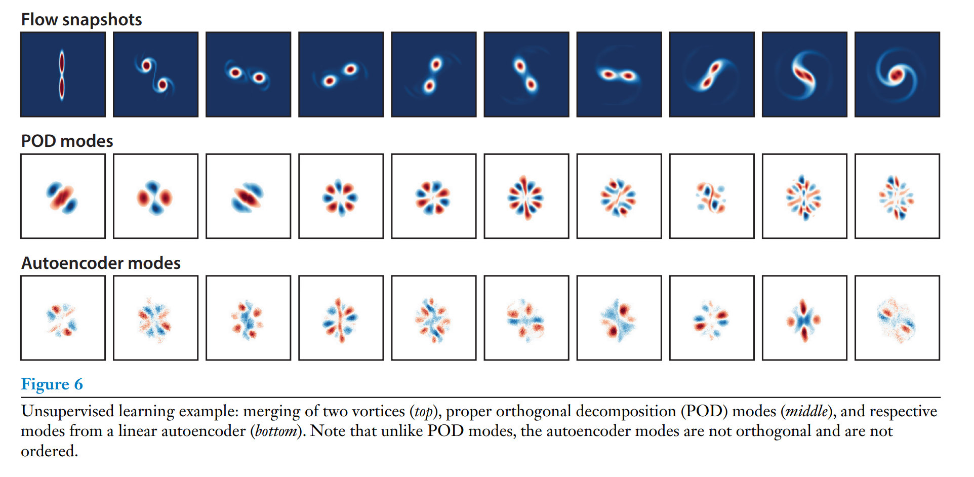
POD is closely related to the algorithm of PCA, one of the fundamental algorithms of applied statistics and ML, to describe correlations in high-dimensional data. We recall that the PCA can be expressed as a two-layer neural network, called an autoencoder, to compress high-dimensional data for a compact representation, as shown in Figure 5. This network embeds high-dimensional data into a low-dimensional latent space and then decodes from the latent space back to the original high-dimensional space. When the network nodes are linear and the encoder and decoder are constrained to be transposes of one another, the autoencoder is closely related to the standard POD/PCA decomposition (Baldi & Hornik 1989) (see also Figure 6).  However, the structure of the NN autoencoder is modular, and by using nonlinear activation units for the nodes, it is possible to develop nonlinear embeddings, potentially providing more compact coordinates. This observation led to the development of one of the first applications of deep NNs to reconstruct the near-wall velocity field in a turbulent channel flow using wall pressure and shear (Milano & Koumoutsakos 2002). More powerful autoencoders are available today in the ML community, and this link deserves further exploration. 

On the basis of the universal approximation theorem (Hornik et al. 1989), which states that a sufficiently large NN can represent an arbitrarily complex input-output function, deep NNs are increasingly used to obtain more effective nonlinear coordinates for complex flows. However, deep learning often imples the availability of large volumes of training data that far exceed the parameters of the network. The resulting models are usually good for interpolation but may not be suitable for extrapolation when the new input data have different probability distributions than the training data (see Equation 1). In many modern ML applications, such as image classification, the training data are so vast that it is natural to expect that most future classification tasks will fall within an interpolation of the training data. For example, the ImageNet data set in 2012 (Krizhevsky et al. 2012) contained over 15 million labeled images, which sparked the current movement in deep learning (LeCun et al. 2015). Despite the abundance of data from experiments and simulations, the fluid mechanics community is still distanced from this working paradigm. However, it may be possible in the coming years to curate large, labeled, and complete-enough fluid databases to facilitate the deployment of such deep learning algorithms. 

유체역학 시뮬레이션과 모델링에서 일반적인 접근 방식은 물리적 좌표를 모달 기저(modal basis)로 변환하는 선형 직교 변환을 정의하는것이다. POD(Proper Orthogonal Decomposition)는 경험적 측정을 기반으로 복잡한 기하 구조에 대한 직교 기저을 제공한다. Sirovich는 1987년 Snapshot POD를 발표했는데, 이건 데이터 중심 방식으로 계산을 간소화하며, 특이값 분해(SVD, Singular Value Decomposition)를 사용해 구현된다. 흥미롭게도 같은 해에 Sirovich는 POD를 이용해 사람 얼굴의 저차원의 공간적 특징을 생성해 오늘날 컴퓨터 비전의 기반이 되는 것을 개발하였다. 

POD는 PCA의 알고리즘과 밀접해 있는데, 이것은 고차원의 데이터를 상관성을 설명하는 데 사용되는 통계 및 ML의 기본 알고리즘이다. PCA는 2층 신경망(autoencoder)으로 표현될 수 있고, 이것은 저차원의 잠재 공간(latent space)으로 임베딩한 후 원래의고차원 공간으로 다시 디코딩한다(Figure 5 참조). 이때, 네트워크 노드가 선형이고 인코더와 디코더가 서로 전채 행렬일 경우(constrained to be transposes of one another), autoencoder는 표준 POD/PCA 분해와 밀접한 관련된다 (Figure 6 참고).  NN 인코더의 구조는 모듈 형식이어서 노드에 비선형의 액티베이션 유닛을 사용하면 비선형 활성화 함수가 적용된 autoencoder를 사용하면 더 압축된 비선형 임베딩의 개발이 가능하다.  최초의 심층NN의 응용 사례 중 하나는 벽면의 압력과 전단 응력을 사용해 난류 채널 흐름의 근벽 속도장을 복원하는 작업이었다. 현재는 더욱 강력한 autoencoder들이 개발되어, 이러한 기술을 유체 역학에 활용할 가능성이 더욱 커졌다.

심층 신경망은 보편 근사 정리(Universal Approximation Theorem,Hornik et al., 1989)에 따르면 복잡한 입력-출력 관계를 나타낼 수 있다. 이를 통해 복잡한 유동 현상에 대해 더 효과적인 비선형 좌표를 생성할 수 있다. 하지만, 딥러닝을 일반적으로 네트워크의 매개변수를 초과할 정도로 대량의 학습 데이터를 필요로 한다. 훈련 데이터 분포와다른 입력 데이터가 제공될 경우, 딥 러닝 모델은 외삽(extrapolation)에서 성능이 저하될 수 있다(Equation 1 참고). 이미지 분류와 같은 최근의 ML 응용법에서 학습 데이터의 양은 방대해서 미래에 분류 작업에 들어오는 데이터가 학습 데이터 안에서 찾아질 것이라고 여겨지는것이 가능하다. 예를 들자면, 2012년에 만들어진 ImageNet 데이터 셋은 1,500만개의 라벨링된 이미지를 포함하고 있었고 이것이 현재의 딥러닝 흐름을 만들었다고 한다. 하지만 실험과시뮬레이션의 풍족함에도 불구하고, 유체 역학 커뮤니티는 이러한 작동 패러다임에서 동떨어져 있다. 하지만, 몇년 후에는 방대한 라벨링 된 그리고 완료된 유체 데이터베이스를  사용해 그러한 심층 학습 알고리즘을 실행시키는것이 가능하게 될 수도 있다. 

3.1.2. 클러스터링과 분류

Clustering ans classification are cornerstones of ML. There are dozens of mature algorithms to choose from, depending on the size of the data and the desired number of categories. The k-means algorithms has been successfully employed by Kaiser et al.(2014) to develop a data-driven discretization of a high-dimensional phase space for the fluid mixing layer. This low-dimensional representation, in terms of a small number of clusters, enabled tractable Markov transition models of how the flow evolves in time from one state to another. Because the cluster centroids exist in the data space, it is possible to associate each cluster centroid with a physical flow fields, lending additional interpretability. Amsallem et al.(2012) used k-means clustering to partition phase space into separate regions, in which local reduced-order bases were constructed, resulting in improved stability and robustness to parameter variations. 

Classification is also widely used in fluid dynamics to distinguish between various canonical behaviors and dynamic regimes. Classification is a supervised learning approach where labeled data are used to develop a model to sort new data into one of several categories. Recently, Colvert et al.(2018) investigated the classification of wake topology (e.g., 2S,2P + 2S, 2P + 4S) behind a pitching airfoil from local vorticity measurements using NNs; extensions have compared performance for various types of sensors (Alsalman et al. 2018). Wang & Hemati (2017) used the k-nearest-neighbors algorithm to detect exotic wakes. Similarly, NNs have been combined with dynamical systems models to detect flow distrurbaces and estimate their parameters (Hou et al. 2019). Related graph and network approaches in fluids by Nair & Taira (2015) have been used for community detection in wake flows (Meena et al. 2018). Finally, one of the earliest examples of ML classification in fluid dynamics by Bright et al. (2013) was based on sparse representation (Wright et al. 2009). 

클러스터링과 분류는 ML의 핵심 요소로, 데이터의 크기와 원하는 범주의 수에 따라  다양한 알고리즘이 활용될 수 있다. K-수 알고리즘의 성공적인 응용 사례로 Kaiser et al.(2014)의 고차원 유체 혼합층의 위상 공간을 데이터 기반으로 이산화한 것이 있다. 이러한 적은수의 클러스터로 표현된 저차원 모델은 시간에 따른 흐름의 상태 변화를 설명하는 마코프 전이(Markov transition) 모델의 개발을 가능하게 만들었다. 클러스터의 중심(centroid)은 데이터 공간에 존재하기 때문에, 각각의 중심을 특정 물리적인 유동 필드와 연결할 수 있어 해석에 유용하다. 2012년, Ansallem et al.이 k-수 클러스터링을 이용해 위상 공간을 여러지역으로 나누고, 각 지역에서 지역적 저차원 기저(local reduced-order bases)를 구성해 매개변수의 변화에 안성성과 견고성을 개선하였다. 

분류는 유체역학에서 보편적으로 사용되는데, 다양한 표준이 되는 행동과 동적 영역의 구분을 하기 위해 사용된다. 분류는 라벨링된 데이터를 사용해 새로운 데이터를 많은 카테고리중의 하나로 분류하는 모델을 개발하는데 사용되는 지도 학습법이다. 최근에, Clovert et al.(2018)는 NN을 활용해 피칭 에어포일(pitching airfoil)후류의 위상 분류(예: 2S,2P + 2S, 2P + 4S)를 위해 국소 와도(vorticity) 측정을 기반하였고 이후 연구에서는 다양한 유형의 센서를 비교해 성능을 평가하였다. 2017년 Wang & Hemati는 k-근접 이웃 알고리즘을 사용해 이례적인 후류 탐지하는데 사용하였다. 그와 비슷하게, Hou et al.(2019)는 NN과 동역학 모델을 결합해 유동 교란(flow disrutbance)을 감지하고 관련된 매개변수를 예측하는데 사용되었다. Nair & Taira(2015)는 그래프이론을 활용해 유체의 네트워크 커뮤니티를 사용했으여, Meena et al.(2018)은 이를 후류 흐름에 적용하였다. 마지막으로, Bright et al.(2013)은 희소 표현(sparse representation)을 사용한 초기 ML 분류 사례로, 이는 Wright et al.(2009) 기초하였다.

3.1.3. 희소및 랜덤화 기법

In parallel to ML, there have been greate strides in sparse optimization and radomized linear algebra. ML and sparse algorithms are synergistic in that underlying low-dimensional representations facilitate sparse measurements (Manohar et al. 2018) and fast randomized computations (Halko et al. 2011). Decreasing the amount of data to train and execute a model is important when a fast decision is required, as in control. In this context, algorithms for the efficient acquisition and reconstruction of sparse signals, such as compressed sensing (Donoho 2006), have already been leveraged for compact representations of wall-bounded turbulence (Bourguignon et al. 2014) and for POD-based flow reconstruction (Bai et al. 2014). 

Low-dimensional structure in data also facilitates accelerated computations via randomized linear algebra (Halko et al. 2011, Mahoney 2011). If a matrix has low-rank structure, then there are efficient matrix decomposition algorithms based on random sampling; this is closely related to the idea of sparsity and the high-dimensional geometry of sparse vectors. The basic idea is that if a large matrix has low-dimensional structure, then with high probability this structure will be preserved after projecting the columns or rows onto a random low-dimensional subspace, facilitating efficient downstream computations. These so-called randomized numerical methods have the potential to transform computational linear algebra, proving accurate matrix decompositions at a fraction of the cost of deterministic methods. For example, randomized linear algebra may be used to efficiently compute the singular value decomposition, which is used to compute PCA (Rokhlin et al. 2009, Halko et al. 2011). 

ML과 병행하며, 희소 최적화와 랜덤화 선형 대수 분야에서도 굉장한 발전이 이루어졌다. 이러한 기법들은 ML과 상호보완적으로 작용해, 저차원의 표현이 희소 측정을 용이하게 하고 빠른 랜덤한 계산을 가능하게 한다. 빠른 의사결정이 필요한 상황(예:제어)에서는 모델을 학습하고 실행하는데 데이터의 양을 줄이는것이 중요하다. 이러한 맥락에서, 압축 센싱(Compressed Sensing)과 같은 희소 시그널들을 효율적으로 수집하고 재구성하는 알고리즘이다. 압축 센싱은 벽 제약 난류(wall-bounded turbulence)의 압축 표현해 사용되었고 (Bourguignon et al. 2014), POD 기반 유동 재구성을 위한 효과적인 도구로도 활용되었다 (Bai et al. 2014).

데이터에서 저차원 구조는 랜덤화 선형 대수를 통해 계산을 가속화할 수 있다 (Halko et al. 2011, Mahoney 2011). 만약 행렬이 저계수 구조(low-rank structure)를 가진다면, 랜덤 샘플링 기반의 효율적인 행렬 분해 알고리즘의 적용이 가능하다. 이 접근법은 희소성 및 희소 벡터의 고차원의 기하학적 구조와 긴밀하게 연괸이 되어 있다. 랜덤화 선형 대수의 핵습 아이디어는 큰 행렬이 저차원의 구조를 갖고 있다면, 열(column) 또는 행(row)을 랜덤 저차원 서브스페이스로 투영해도 높은 확률로 그 구조가 보존된다. 이를 통한 효율적인 후속 계산이 가능하다. 랜덤화 수치 기법은 기존의 결정론적 방법보다 훨씬 적은 비용으로 정확한 행렬 분해를 제공한다. 응용 사례로는 특잇값 분해(SVD,singular value decomposition)가 있는데, 이것은 PCA를 계산하는 데 사용되며, 랜덤화 선형 대수를 통해 더욱 효율적으로 구현할 수 있다 (Rokhlin et al. 2009, Halko et al. 2011).

3.1.4. 초해상도 및 유동 정화

Much of ML is focused on imaging science, providing robust approaches to improve resolution and remove noise and corruption based on statistical inference. These supreresolution and denoising algorithms have the potential to improve the quality of both simulations and experiments in fluids. 

Superresolution involves the inference of a high-resolution image from low-resolution measurements, leveraging the statistical structure of high-resolution training data. Several approaches have been developed for superresolution, for example, based on a library of examples (Freeman et al. 2002), sparse representation in a library (Yang et al. 2010), and most recently CNNs (Dong et al. 2014). Experimental flow field measurements from PIV (Adrian 1991, Willert & Gharib 1991) provide a compelling application where there is a tension between local flow resolution and the size of the imaging domain. Superresolution could leverage expensive and high-resolution data on smaller domains to improve the resolution on a larger imaging domain. Large-eddy simulations(LES) (Germano et al. 1991, Meneveau & Katz 2000) may also benefit from superresolution to infer the high-resolution structure inside a low-resolution cell that is required to compute boundary contitions. Recently, Fukami et al. (2018) developed a CNN-based superresolution algorithm and demonstrated its effectiveness on turbulent flow reconstruction, showing that the energy spectrum is accurately preserved. One drawback of superresolution is that it is often extremely costly computationally, making it useful for applications where high-resolution imaging may be prohibitively expensive; however, improved NN-based approaches may drive the cost down significantly. We note also that Xie et al. (2018) recently employed GANs for superresolution. 

The processing of experimental PIV and particle tracking has also been one of the first applications of ML. NNs have been used for fast PIV (Knaak et al. 1997) and PTV ((Labonté 1999), with impressive demonstrations for three-dimensional Lagrangian particle tracking (Ouellette et al. 2006). More recently, deep CNNs have been used to construct velocity fields from PIV image pairs (Lee et al. 2017). Related approaches have also been used to detect spurious vectors in PIV data (Liang et al. 2003) to remove outliers and fill in corrupt pixels. 

ML의 많은 연구는 영상 과학에 중점을 두고 있으며, 통계적 추론을 기반으로 해상도를 향상시키고 잡음과 왜곡을 제거하는 강력한 접근법을 제공한다. 이러한 초해상도 및 잡음 제거 알고리즘은 유체 시뮬레이션과 실험의 질을 개선시킬 수 있는 가능성이 있다. 

초해상도는 저해상도 측정값으로부터 고해상도 이미지를 추론하는 기술로, 고해상도 훈련 데이터의 통계적 구조를 활용한다. 초해상도의 기존 접근법에는, 예제 라이브러리를 기반으로 한 방법 (Freeman et al. 2002), 희소 표현 라이브러리를 활용한 방법 (Yang et al. 2010), 그리고 최근의 합성곱 신경망 (CNN) 기반 방법 (Dong et al. 2014)이 있다. 적용 사례로는 입자 영상 속도계(PIV; Adrian 1991, Willert & Gharib 1991) 데이터를 활용한 초해상도는 국부의 유동 해상도와 영상 도메인 크기 사이의 균형 문제를 해결할 수 있다. 다른 사례로는 고가의 고해상도 데이터를 작은 영역에서 수집한 후, 이를 사용해 더 큰 영상 영역의 해상도를 향상시킬 수 있다. 대와류 시뮬레이션 (LES, Large-eddy simulations)을 사용해 저해상도 셀 내부의 고해상도 구조를 추론해 경계 조건 계산에 필요한 데이터를 제공할 수 있다. 최근 연구로는 Fukami et al.(2018)이 CNN 기반의 초해상도 알고리즘을 개발해 난류 재구성에서의 효과성을 증명하여 에너지 스펙트럼이 정확히 보존되는걸 보여주었다.초해상도의 단점으로는 계산하는 비용이 매우 높아, 고해상도 이미징이 지나치게 비싼 응용 분야에서 유용하게 사용된다는 것이다. 하지만, 향상된 NN 기반의 접근법은 비용을 크게 줄이는것이 가능하다. 또한 Xie et al.(2018)은 생성적 적대 신경망(GAN)을 활용한 초해상도 기술을 도입하기도 하였다.

입자 영상 속도계(PIV)와 입자 추적(PTV) 데이터 처리는 ML의 초기 응용법 중 하나였다. 초기 연구로는 신경망(NN)을 활용한 빠른 PIV 처리 (Knaak et al. 1997), 입자 추적(PTV) (Labonté 1999), 3차원 라그랑지안 입자 추적(Ouellette et al. 2006)에서 인상적인 성과기 있다. 최근 연구로는 심층 CNN을 활용해 PIV 이미지 페어에서 속도장을 구성하는데 사용되기도 했다. 관련된 접근법들은 PIV 데이터에서 거스퓨리어스 벡터(spurious vector)를 탐지해 이상치와 손상된 픽셀을 제거하는데 사용되기도 했다. 

3.2. 유체 역학 모델링하기

A central goal of modeling is to balance efficiency and accuracy. When modeling physical systems, interpretability and generalizability are also critical considerations. 

모델링에서의 중심 목표는 효율성과 정확성의 균형을 맞추는 것이다. 물리 시스템을 모델링할 때, 해석 가능성과 일반화 가능성 또한 주요한 고려 대상이 될 것이다. 

3.2.1. 비선형 임베딩으로 통한 선형 모델: 동적 모드 분해(DMD)와 쿠프만 분석

Many classical techniques in system identification may be considered ML, as they are data-driven models that generalize beyond the training data. Dynamic mode decomposition (DMD) (Schmid 2010, Kutz et al. 2016) is a modern approach to extract spatiotemporal coherent structures from time series data of fluid flows, resulting in a low-dimensional linear model for the evolution of these dominant coherent structures. DMD is based in data-driven regression and is equally valid for time-resolved experimental and numerical data. DMD is closely related to the Koopman operator (Rowley et al. 2009, Mezic 2013), which is an infinite-dimensional linear operator that describes how all measurement functions of the system evolve in time. Because the DMD algorithm is based in linear flow field measurements (i.e., direct measurements of the fluid velocity or vorticity field), the resulting models may not be able to capture nonlinear transients. 

Recently, there has been a concerted effort to identify a coordinate system where the nonlinear dynamics appears linear. The extended DMD (Williams et al. 2015) and variational approach of conformation dynamics (Noé & Nüske 2013, Nüske et al. 2016) enrich the model with nonlinear measurements, leveraging kernel methods (Williams et al. 2015) and dictionary learning (Li et al. 2017). These special nonlinear measurements are generally challenging to represent, and deep learning architectures are now used to identify nonlinear Koopman coordinate systems where the dynamics appear linear (Takeishi et al. 2017, Lusch et al. 2018, Mardt et al. 2018, Wehmeyer & Noé 2018). The VAMPnet architecture (Mardt et al. 2018, Wehmeyer & Noé 2018) uses a time-lagged autoencoder and a custom variational score to identify Koopman coordinates on an impressive protein folding example. Based on the the performance of VAMPnet, fluid dynamics may benefit from neighboring fields, such as molecular dynamics, which have similar modeling issues, including stochasticity, coarse-grained dynamics, and separation of timescales. 

많은 고전적 시스템 식별 기법은 데이터 기반 모델로, 학습 데이터를 나아가 일반화할 수 있다는 점에서 ML의 일부로 간주될 수 있다. 동역학 모드 분해(DMD, Dynamic Mode Decomposition)는 Schmid(2010)과 Kutz et al.(2016)에 의해 소개된 현대적 접근법으로, 유동 데이터의 시계열에서 시공간적 연계 구조를 추출해 이러한 구조의 진화를 설명하는 저차원 선형 모델을 생성한다. DMD는 데이터 기반 회귀법에 기반되어 있고, 시간에 따른 실험적 데이터와 수치 데이터를 모두 처리할 수 있다. DMD는 쿠프만 연산자와 밀접한 관련이 있는데, 이것은 시스템의 모든 측정 함수가 시간에 따라 어떻게 진화하는지 설명하는 무한 차원의 선형 연산자이다. 그러나 DMD 알고리즘은 유체 속도장이나 와도장의 선형 측정값 기반하기 때문에 , 결과적으로 나온 모델은 비선형 과도 현상을 포착하지 못할 수 있다. 

최근 들어서 비선형 동역학이 선형적으로 보이는 좌표계를 식별하려는 노력이 강화되었다. 향상된 모델 기법으로 비선형 측정값을 모델에 추가하여 커널 기법과 사전 학습된 사전을 활용하는 Extended DMD와 비선형 측정값을 활용하여 동역학을 더 풍부하게 표현하는 변분 접근법이 있다. 딥러닝을 활용한 비선형 좌표계 식별을 위해 Takeishi et al. (2017), Lusch et al. (2018), Mardt et al. (2018), Wehmeyer & Noé (2018)의 연구들은 비선형 쿠프만 좌표계를 찾기 위해 딥러닝 구조를 도입하였다. VAMPnet 구조는 시간 지연(autoencoder)과 커스텀 변분 점수를 사용해 좌표를 식별한다.이 기술은 단백질 접힘과 같은 예제에서 뛰어난 성과를 보였다. VAMPnet의 성능에 기반해서, 유체 역학은 확률성과 거칠게 구분된 동역학, 그리고 시간 척도의 분리 등 유사한 모델링 문제가 있는 분자 역학과 같은 이웃의 분야에서 배울 점이 많다.

3.2.2. 신경 네트워크(NN) 모델링

Over the last three decades, NNs have been used to model dynamical systems and fluid mechanics problems. Early examples include the use of NNs to learn the solutions of ordinary and partial differential equations (Dissanayake & Phan-Thien 1994, Gonzalez-Garcia et al. 1998, Lagaris et al. 1998). We note that the potential of these works has not been fully explored, and in recent years there have been further advances (Chen et al. 2018, Raissi & Karniadakis 2018), including discrete and continuous-in-time networks. We note also the possibility of using these methods to uncover latent variables and reduce the number of parametric studies often associated with partial differential equations (Raissi et al. 2019). NNs are also frequently employed in nonlinear system identification techniques such as NARMAX, which are often used to model fluid systems (Glaz et al. 2010, Semeraro et al. 2016). In fluid mechanics, NNs were widely used to model heat transfer (Janbunathan et al. 1996), turbomachinery (Pierret & Van den Braembussche 1999), turbulent flows (Milano & Koumoutsalos 2002), and other problems in aeronautics (Faller & Schreck 1996). 

RNNs with LSTMs (Hochreiter & Schmidhuber 1997) have been revolutionary for speech recognition, and they are considered one of the landmark success of AI. They are currently being used to model dynamical systems and for data-driven predictions of extreme events (Vlachas et al. 2018, Wan et al. 2018). An interesting finding of these studies is that combining data-driven and reduced-order models is a potent method that outperforms each of its components on several studies. GANs (Goodfellow et al. 2014) are also being used to capture physics (Wu et al. 2018). GANS have potential to aid in the modeling and simulation of turbulence (Kim et al. 2018), although this field is nascent. 

Despite the promise and widespread use of NNs in dynamical systems, several challenges remain. NNs are fundamentally interpolative, and so the function is well approximated only in the span (or under the probability distribution) of the sampled data used to train them. Thus, caution should be exercised when using NN models for an extrapolation task. In many computer vision and speech recognition examples, the training data are so vast that nearly all future tasks may be viewed as an interpolation on the training data, although this scale of training has not been achieved to date in fluid mechanics. Similarly, NN models are prone to overfitting, and care must be taken to cross-validate models on a sufficiently chosen test set; best practices are discussed by Goodfellow et al. (2016). Finally, it is important to explicitly incorporate partially know physics, such as symmetries, constraints, and conserved quantities. 

지난 30년 동안, NN은 동역학 시스템과 유체 역학 문제를 모델링하는 데 푸는데 사용되었다. 초기 연구로는 상미분 방정식(ODE) 및 편미분 방정식(PDE)의 해를 학습하기 위한 NN의 활용이 있었다. 이러한 연구들의 잠재력은 아직 완전히 탐구되지 않았으며, 최근 들어 더 발전된 연구가 진행되고 있다. 여기에는 시간 불연속 및 연속 신경망이 포함되는데, 잠재 변수를 발견하거나 PDE와 관련된 매개변수 연구의 필요성을 이러한 방법이 사용됨으로 인해 내재된 다양성들과 매개변수의 수를 줄이는 가능성도 제시된다. NN은 또한 NARMAX와 같은 비선형 시스템 알아내는 기법에서 사용되어 유체 시스템의 모델링하는데 사용되기도 한다. 유체역학에서 NN은 열 전달 모델이나 터보머신 설계, 난류흐름 모델링이나 다른 공기역학 문제을 만들기 위해 사용되었다. 

LSTM과 결합한 RNN은 음성 인식에 있어 혁명적이었고 AI의 성공에 있어 하나의 지표점이 되었다. 이것들은 현재 극한 사건의 데이터 기반 예측을 위한 동역학 시스템 모델링에 사용되었다. 이러한 연구들은 데이터 기반 모델과 저차원 모델을 결합하는 것에 개별 요소를 능가하는 강력한 방법임을 보여준다. GAN은 물리적 현상을 포착하기 위해 사용되고 있으며, 특히 난류의 모델링 및 시뮬레이션에서 잠재력을 보여주고 있다. 

NN이 가진 가능성에도 불구하고, 여러 도전 과제가 존재한다. NN은 주어진 훈련 데이터의 확률 분포 내에서만 정확한 근사를 제공한다. 따라서 NN 모델을 외삽 작업에 사용할 때는 신중해야 한다. 많은 컴퓨터 비전과 음성 인식 예시에서는 학습 데이터가 방대하기 때문에 대부분의 미래 작업이 학습 데이터의 보간으로 간주될 수 있지만, 이러한 사이즈의 학습은 유체 역학에서는 아직 도달되지 않았다. 비슷하게, NN 모델은 과적합에 취약하며, 효과적으로 선택된 테스트 세트를 통해 교차 검증을 수행해야 한다. Goodfellow et al.(2016)은 이에 대한 모범 사례를 논의한다. 대칭성, 제약 조건, 보존 법칙과 같은 부분적으로 알려진 물리적 법칙을 명시적으로 통합하는 것이 중요하다고 할 수 있다.

3.2.3. 간결한 비선형 모델

Parsimony is a recurring theme in mathematical physics, from Hamilton's principle of least action to the apparent simplicity of many governing equations. In contrast to the raw representational power of NNs, ML algorithms are also being employed to identify minimal models that balance predictive accuracy with model complexity, preventing overfitting and promoting interpretability and generalizability. Genetic programming was recently used to discover conservation laws and governing equations (Schmidt & Lipson 2009). Sparse regression in a library of candidate models has also been proposed to identify dynamical systems (Bruntom et al. 2016) and partial differential equations (Rudy et al. 2017, Schaeffer 2017). Loiseau & Brunton (2018) identified sparse reduced-order models of several flow systems, enforcing energy conservation as a constraint. In both genetic programming and sparse identification, a Pareto analysys is used to identify models that have the best trade-off between model complexity, measured in number of terms, and predictive accuracy. In cases where the physics is known, this approach typically discovers the correct governing equations, proving exceptional generalizability compared with other leading algorithms in ML. 

간결성(parsimony)는 수학 물리학의 핵심 주제로, 해밀턴의 최소 작용 원리에서부터 많은 지배 방정식의 명백한 단순성에 이르기까지 다양하게 나타난다. NN의 강력한 표현 능역과는 대조적으로, ML 알고리즘은 예측 정확성과 모델 복잡성 간의 균형을 맞추기 위해 최소 모델(minimal models)을 식별하는 데도 활용되고 있다. 이는 과적합을 방지하고, 모델의 해석 가능성과 일반화 가능성을 촉진라는데 도움을 준다. Schmidt & Lipson (2009)은 보존 법칙과 지배 방정식을 발견하기 위해 유전 사용하였다. 희소 회귀 접근 방식으로는 후보 모델의 라이브러리에서 희소 회귀를 사용해 동역학 시스템과 편비분 방정식(PDE)을 식별하는 방법이 제안되었다. Loiseau & Brunton(2018)은 여러 유동 시스템의 희소 저차원 모델을 식별하는 데 성공했으며, 이 과정에서 에너지 보존을 제약 조건으로 사용하였다. 파레토 분석(Pareto Analysis)은 모델 복잡성과 예측 정확성 간의 최적 균형을 이루는 모델을 식별하는 데 사용된다. 여기서 모델 복잡성은 방정식의 항(term) 개수로 측정되고, 예측 정확성은 모델의 데이터 적합성을 평가한다. 물리적 법칙이 이미 알려진 경우, 이러한 접근 방식은 일반적으로 정확한 지배 방정식을 발견해, 다른 ML의 방정식에 비교해서 탁월한 일반화 능력을 제공한다.

3.2.4. 머신 러닝을 활용한 클러저 모델

The use of ML to develop turbulence closures is an active area of research (Duraisamy et al. 2019). The extreme separation of spatiotemporal scales in turbulent flows makes it exceedingly costly to resolve all scales in simulation, and even with Moore's law, we are decades away from resolving all scales in relevant configurations (e.g., aricraft, submarines, etc). It is common to truncate small scales and model their effect on the large scales with a closure model. However, these models may require careful tuning to match data from fully resolved simuations or experiments. 

ML has been used to identify and model discrepancies in the Reynolds stress tensor between a RANS model and high-fidelity simulations (Ling & Templeton 2015, Parish & Duraisamy 2016, Ling et al. 2016b, Xiao et al. 2016, Singh et al. 2017, Wang et al. 2017). Ling & Templeton (2015) compared SVMs, Adaboost decision trees, and random forests to classify and predict regions of high uncertainty in the Reynolds stress tensor. Wang et al. (2017) used random forests to build a supervised model for the discrepancy in the Reynolds stress tensor. Xiao et al. (2016) leveraged sparse online velocity measurements in a Bayesian framework to infer these discrepancies. In related work, Parish & Duraisamy (2016) developed the field incersion and ML modeling framework that builds corrective models based on inverse modeling. This framework was later used by Singh et al. (2017) to develop an NN enhanced correction to the Spalart-Allmaras RANS model, with excellent performance. A key result by Long et al. (2016b) employed the forst deep network architecture with many hidden layers to model the anistropic Reynolds stress tensor, as shown in Figure 7. Their novel architecture incorporates a multiplocative layer to embed Galilean invariance into the tensor predictions. This provides an innovative and simple approach to embed known physical symmetries and invariances into the learning architecture (Ling et al. 2016a), which we believe will be essential in future efforts that combine learning for physics. For LES closures, Maulik et al. (2019) have employed artificial NNs to predict the turbulence source term from coarsely resolved quantities. 

난류 클로저 모델 개발을 위한 ML의 활용은 현재 활발히 연구되고 있는 분야이다. 난류 유동은 극도로 복잡한 시공간적 규모를 가지며, 모든 스케일을 시뮬레이션으로 해결하기에는 엄청난 비용이 소모된다. 심지어 무어의 법칙을 고려하더라도, 항공기나 잠수함과 같은 실제 환경에서 모든 스케일을 해결하기까지는 수십 년이 소요될 것으로 예상된다. 작은 스케일을 생략하고, 이들이 큰 스케일에 미치는 영향을 클로저 모델을 통해 나타내는 방식이 일반적이다. 

대표적인 접근법으로는 레이놀즈 평균 나비에-스토크스 방정식(RANS) 및 대와류 시뮬레이션(LES)이 있다. 그러나 이러한 모델들은 종종 고해상도 시뮬레이션 또는 실험 데이터를 기반으로 하는 신중한 조정이 필요하다. 모신러닝을 활용한 난류 모델 개선 사례에는 레이놀즈 응력 텐서(RST) 불일치 식별 및 모델링, 역모델링 기반 수정 모델 개발, 심층 신경망을 활용한 난류 응력 텐서 모델링, 그리고 LES 클로저 모델링이 있다. ML은 RANS 모델과 고해상도 시뮬레이션 간의 레이놀즈 응력 텐서 불일치를 식별하고 모델링하는데 사용되었다. Ling & Templeton (2015)는 서포트 벡터 머신(SVM)과 Adaboost 결정 트리, 그리고 랜덤 포레스트를 활용해 레이놀즈 응력 텐서의 높은 불확실성 영역을 분류하고 예측하였다. Wang et al. (2017)은 랜덤 포레스트를 사용해 RST 불일치를 모델링하는 지도 학습 모델을 구축하였고, Xiao et al.(2016)은 희소한 온라인 속도 측정을 베이시안 프레임워크로 통합해 불일치를 추론하였다. 역모델링 기반 수정 모델 개발 연구로는, Parish & Duraisamy (2016)의 역모델링을 기반으로 수정 모델을 개발하는 필드 반전 및 ML 모델링 프레임워크 제안과, Singh et al. (2017)의 Spalart-Allmaras RANS 모델의 NN 기반 보정 모델 개발이 있다. 심층 신경망을 활용한 난류 응력 텐서 모델링으로는 Figure 7에서 볼 수 있듯이,  Long et al. (2016b)의 다중 은닉층을 가진 최초의 심층 신경망 구조를 사용한 비등방성 레이놀즈 응력 텐서 모델링이 있는데, 여기에서는 갈릴레이 불변성(Galilean Invariance)을 텐서 예측에 통합하는 곱셈 계릉을 설계해, 물리적 대칭성과 불변성을 학습 구조에 내재하였다. LES 클로저 모델링으로는 Maulik et al. (2019)의 인공 신경망을 사용한 낮은 해상도 변수로부터 난류 소스 항을 예측한 연구가 있다.

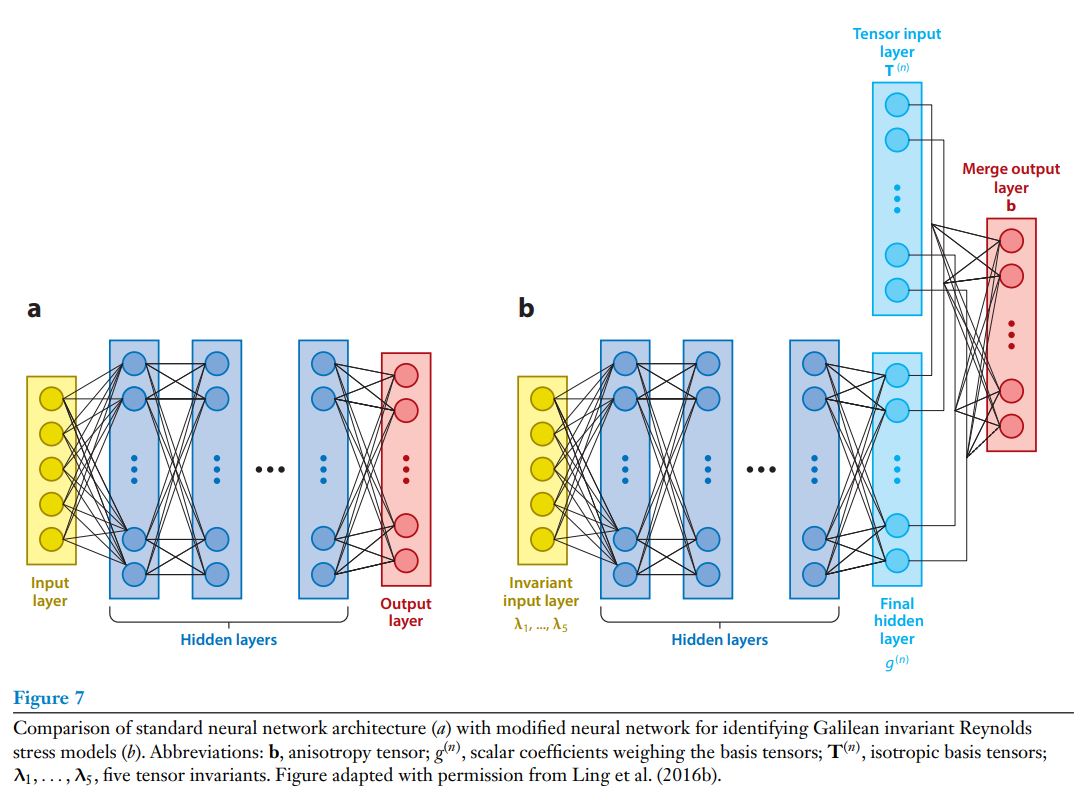
3.2.5. 동적 시스템에 ML을 적용하는데 있어서의 도전 과제

Applying ML to model physical dynamical systems poses several unique challenges and opportunities. Model interpretability and generalizability are essential cornerstones in physics. A well-crafted model will yield hypothises for phenomena that have not been observed before. This principle is for example exhibited in the parsimonious formulation of classical mechanics in Newton's second law. 

High-dimensional systems, such as those encountered in unsteady fluid dynamics, have the challenges of multiscale dynamics, sensitivity to noise and disturbances, latent variables, and transients, all of which require careful attention when applying ML techniques. In ML for dynamics, we distinguish two tasks: discovering unknown physics and improving models by incorporating known physics. Many learning architectures cannot readily incorporate physical constraints in the form of symmetries, boundary conditions, and global conservation laws. This is a critical area for continued development, and several recent works have presented generalizable physics models (Battaglia et al. 2018). 

물리적 동적 시스템을 모델링하기 위해 ML 을 적용하는 것은 독특한 도전 과제와 기회를 제공한다. 모델의 해석 가능성과 일반화 가능성은 물리학의 필수적인 요소이다. 잘 설계된 모델은 아직 관찰되지 않은 현상에 대한 가설을 도출할 수 있어야 하며, 이는 뉴턴의 제 2 법칙처럼 간결하게 표현된 고전 역학의 원리에서도 관측될 수 있다. 

비정상 유체역과 같은 고차원의 시스템에서는 다중 스케일 동역학과 같은 서로 다른 시공간 규모에서 상호작용하는 복잡한 현상, 노이즈와 교란에 대한 민감성, 시스템에 내재하지만 직접 관찰되지 않은 잠재 변수, 그리고 시스템이 안정 상태로 전환되기 전 나타나는 임시적이고 복잡한 과도 현상과 같은 어려움이 존재한다. 이러한 요소들은 ML 기법을 적용할 때 세심한 주의가 필요된다. ML을 동적 시스템에 적용하는 데는 다음 두 가지의 주요 작업이 있는데, 하나는 데이터를 기반으로 새로운 물리적 현상을 이해하고 설명하는 모델을 개발하는 것이고, 다른 하나는 기존에 알려지 물리 법칙(예를 들면 대칭성, 경계 조건, 보존 법칙 등)을 통햅해 기존 모델을 개선하는 작업이 필요하다. 대다수의 ML 아키텍처는 대칭성(Symmetries), 경계 조건(Boundary Conditions), 그리고 전역 보존 법칙(Global Consercation Laws)와 같은 물리적 제약을 쉽게 통합하지 못한다. 이 문제는 지속적인 개발이 필요한 핵심 영역으로, 최근 연구들은 이러한 제약을 포함할 수 있는 일반화된 물리 모델을 제시하였다 (Battaglia et al. 2018).

4. 유체 최적화 및 제어에서 머신러닝의 활용 

Learning algorithms are well suited to flow optimization and control problems involving blackbox or multimodal cost functions. These algotithms are iterative and often require several orders of magnitude more cost function evaluations than gradient-based algorithms (Bewley et al. 2001). Moreover, they do not offer guarantees of convergence, and we suggest that they be avoided when techniques such as adjoint methods are applicable. At the same time, techniques such as RL have been shown to outerperform even optimal flow control strategies (Novati et al. 2019). Indeed, there are several classes of flow control and optimization problems where learning algorithms may be the method of choice, as described below.
In contrast to flow modeling, learning algorithms for optimization and control interact with the data sampling process in several ways. First, in line with the modeling efforts described in earlier sections, ML can be applied to develop explicit surrogate models that relate the cost function and the control/optimization parameters. Surrogate models such as NNs can then be amenable to even gradient-based methods, although they often get stuck in local minima. Multifidelity algorithms (Perdikaris et al. 2016) can also be employed to combine surrogates with the cost function of the complete problem. As the learning progresses, new data are requested as guided by the results of the optimization. Alternatively, the optimization or control problem may be described in terms of learning probability distributions of parameters that minimize the cost function. These probability distributions are constructed from cost function samples obtained during the optimization process. Furthermore, the high-dimensional and nonconvex optimization procedures that are currently employed to train nonlinear LMs are well suited to the high-dimensional, nonlinear optimization problems in flow control. 

We remark that the lines between optimization and control are becoming blurred by the availability of powerful computers (see the sidebar titles Optimization and Control: Boundaries Erased by Fast Computers). However, the range of critical spatiotemporal scales and the nonlinearity of the underlyting processes will likely render real-time optimization for flow control a challenge for decades to come. 

머신러닝 알고리즘은 블랙박스 또는 다중 모달 비용 함수를 포함하는 유체 최적화 및 제어 문제를 다루기에 적합하다. 이러한 알고리즘은 반복적으로 작동하며, 종종 기울기 기반 알고리즘보다 수백에서 수천 배의 비용 함수 평가를 필요로 한다(Bewley et al., 2001). 또한, 수렴 보장이 없기 때문에, 인접 방법(adjoints)과 같은 기술이 적용 가능한 경우 머신러닝 알고리즘의 사용을 지양하는 것을 제안한다. 그럼에도 불구하고, 강화 학습과 같은 기법은 심지어 최적의 유체 제어 전략을 초과하는 성과를 보이는 경우도 있다(Novati et al., 2019). 다음에 설명된 바와 같이, 머신러닝 알고리즘이 최선의 선택이 될 수 있는 여러 유형의 유체 제어 및 최적화 문제가 존재한다. 

유체 모델링과 대조되게, 최적화와 제어에 대한 학습 알고리즘은 데이터 샘플링 프로세스와 여러 방식으로 상호작용한다. 첫째로, 앞서 논의된 모델링과 일치하는 방식으로, 머신러닝은 비용 함수와 제어/최적화 매개변수 간의 관계를 명시적으로 나타내는 대리 모델을 개발하는데 활용된다. NN과 같은 대리 모델은 종종 기울기 기반 방법에 적용 가능하지만, 지역 최적값에 갇히는 경우가 많다. Perdikaris et al. (2016)은 대리 모델과 문제의 전체 비용 함수를 결합하기 위해 다중 충실도 알고리즘(multifidelity)을 사용할 수 있음을 제안했다. 학습이 진행됨에 따라 최적화 결과에 의해 새로운 데이터 요청이 이루어진다. 다른 방법으로, 최적화 또는 제어 문제를, 비용 함수를 최소화하는 매개변수의 확률 분포를 학습하는 문제로 정의될 수 있다. 이러한 확률 분포는 최적화 과정에서 얻어잔 비용 함수 샘플로부터 구축된다. 더욱 나아가서, 현재 비선형 머신러닝 모델을 훈련하기 위해 사용되는 고차원, 비볼록(nonconvex) 최적화 절차는 유체 제어에서 발생하는 고차원, 비선형 최적화 문제를 해결하는 데 적합하다. 강력한 컴퓨터의 발전으로 인해 최적화와 제어 사이의 경계는 점점 모호해지고 있다. (Sidebar: 최적화와 제어 참고). 그러나, 유체 제어에서 요구되는 중요한 시공간 스케일의 범위가 기저 프로세스의 비선형성으로 인해 실시간 최적화는 향후 몇십년간 여전히 도전 과제로 남을 가능성이 크다. 

Sidebar: 최적화와 제어: 빠른 컴퓨터가 이 둘의 경계를 허물다

Optimization and control are intimately related, and the boundaries are becoming even less distinct with increasingly fast computers, as summarized by Tsiotras & Mesbahi (2017, p.195):

Interestingly, the distinction between optimization and control is largely semantic and (alas!) implementation-dependent. If one has the capability of solving optimization problems fast enough on the fly to close the loop, then one has (in principle) a feedback control law... Not surprisingly then, the same algorithm can be viewed as solving an optimization or a control problem, based solely on the capabilities of the available hardware. With the continued advent of faster and more capable computer hardware architectures, the boundary between optimization and control will become even more blurred. However, when optimization is embedded in the implementation of feedback control, the classical problems of control such as robustness to model uncertainty, time delays, and process and measurement noise become of paramount importance, particularly for high-performance aerospace systems. 

최적화와 제어는 밀접하게 관련된 분야로, 점점 더 빨라지고 강력해지는 컴퓨터의 발전에 따라 두 개념 간의 경계는 점점 모호해지고 있다. 이에 대해 Tsiotras와 Mesbahi(2017, p.195)는 다음과 같이 요약한다:

"흥미롭게도, 최적화와 제어의 구분은 주로 의미론적 차이와 (불행히도) 구현 방식에 따라 결정된다. 만약 실시간으로 최적화 문제를 충분히 빠르게 해결하여 루프를 닫을 수 있다면, 이는 (원칙적으로) 피드백 제어 법칙이 된다. (중략) 그렇기 때문에, 동일한 알고리즘이 사용 가능한 하드웨어의 성능에 따라 최적화 문제를 해결하는 것으로 볼 수도, 혹은 제어 문제를 해결하는 것으로 볼 수도 있다.점점 더 빠르고 강력한 컴퓨터 하드웨어의 등장으로 인해 최적화와 제어 간의 경계는 더욱 흐릿해지고 있다. 이제는 실시간 최적화가 가능해짐에 따라, 최적화 알고리즘이 곧 피드백 제어 역할을 수행할 수 있다. 하지만 최적화가 피드백 제어에 포함될 경우, 전통적인 제어의 핵심 문제들이 다시 중요해진다. 특히, 고성능 항공우주 시스템에서는 모델 불확실성에 대한 강건성, 시간 지연, 그리고 프로세스 및 측정 노이즈(시스템 동작과 센서 데이터를 방해하는 불확실성)에 대한 문제가 우선적으로 고려되어야 한다."

4.1. 확률적 유체 최적화: 학습 분포 학습

Stochastic optimization includes ES and GAs, which were originally developed based on bio-inspired principles. However, in recent years, these algorithms have been placed in a learning framework (Kern et al. 2004). 

Stochastic optimization has found widespread use in engineering design, in particular as many engineering problems involve black-box-type cost functions. A much-abbreviated list of applications includes aerodynamic shape optimization (Giannakoglou et al. 2006), uninhabited aerial vehicles (UAVs) (Hamdaoui et al. 2010), shape and motion optimization in artificial swimmers (Gazzola et al. 2012, Van Rees et al. 2015), and improved power extraction in crossflow turbines (Strom et al. 2017). We refer readers to the review article by Skinner & Zare-Betash (2018) for an extensive comparison of gradient-based and stochastic optimization algorithms for aerodynamics. 

These algorithms involve large numbers of iterations, and they can benefit from massively parallel computer architectures. Advances in automation have also facilitated their application in experimental (Strom et al. 2017, Martin & Gharib 2018) and industrial settings (Bueche et al. 2002). We note that stochastic optimization algorithms are well suited to address the experimental and industrial challenges associated with uncertainty, such as unexpected behavior, partial descriptions of the system and its environment, and exogenous disturbances. Hansen et al. (2009) proposed an approach to enhance the capabilities of evolutionary algorithms for online optimization of a combustor test rig. 

Stochastic flow optimization will continue to benifit from advances in computer hardware and experimental techniques. At the same time, convergence proofs, explainability, and reliability are outstanding issues that need to be taken into consideration when deploying such algorithms in fluid mechanics problems. Hybrid algorithms that combine in a problem-specific manner stochastic techniques and gradient-based methods may offer the best strategy for flow control problems. 

확률적 최적화(stochastic optimization)는 진화 전략(ES)과 유전 알고리즘(GA)을 포함하는데, 이러한 기법들은 생물학적 용감을 기반으로 초기 개발되었다. 그러나 최근 들어서 이런 알고리즘들은 학습 프레임워크에 포함되게 되었다. 

확률적 최적화는 특히 블랙박스 비용 함수가 포함된 엔지니어링 설계 문제에서 광범위하게 활용되고 있다. 대표적인 적용 사례로는 공기역학적 형상 최적화, 무인 항공기(UAV)의 설계, 인공 수영체의 형상 및 동작 최적화, 그리고 횡류 터빈에서의 전력 추출 향상에 사용되고 있다. 이와 관련된 더 포괄적인 비교는 2018년에 나온 Skinner & Zare-Betash의 항공역학을 위한 그래디언트 기반 확률 최적화 알고리즘의 심화 비교에 대한 글을 읽어보는것을 추천한다.

이러한 알고리즘은 대규모 반복 과정을 수반하기 때문에 병렬 컴퓨터 아키텍처에서 효율적으로 실행될 수 있다. 자동화 기술의 발전은 실험 및 산업 환경에서 확률적 최적화의 적용을 더욱 용이하게 만들었다. 확률적 최적화 알고리즘은 예측하지 못하는 시스템 동작과 시스템 및 그 환경에 대한 불완전한 설명, 그리고 외부 간섭 요인과 같은 불확실성과 연계된 문제를 효과적으로 다루는것이 가능하다. Hansen et al. (2009)은 연소기 시험 장치의 온라인 최적화를 위해 진화 알고리즘의 성능을 향상시키는 접근 방식을 제안하였다. 

확률적 유체 최적화는 컴퓨터 하드웨어와 실험 기술의 발전에 따라 계속해서 진화할 것이다. 그러나 그와 동시에 수렴 증명, 설명가능성, 그리고 신뢰성과 같은 문제들은 항상 고려되어야 하는 부분이다. 또한, 특정 문제에 맞게 확률적 기법과 기울기 기반 방법을 결합한 하이브리드 알고리즘이 유체 제어 문제에서 가장 좋은 전략이 될 가능성이 클 것이다. 

4.2. 유체 제어와 머신 러

Feedback flow control modifies the behavior of a fluid dynamic system through actuation that is informed by sensor measurements. Feedback is necessary to stabilize an unstable system, attenuate sensor noise, and compensate for external disturbances and model uncertainty. Challenges of flow control include a high-dimensional state, nonlinearity, latent variables, and time delays. ML algorithms have been used extensively in control, system identification, and sensor placement. 

피드백 유체 제어는 센서 측정값을 기반으로 한 구동을 통해 유체 역학 시스템의 동작을 수정하는 기법이다. 피드백은 불안정한 시스템의 안정화와 센서 노이즈를 감소시키고, 외부 간섭 및 모델 불확실성 보장을 위해 필요로 한다. 유체 제어의 도전 과제로는 고차원 상태 공간이나 비선형성, 잠재변수, 그리고 시간 지연 등이 있다. ML은 제어 알고리즘 개발이나 시스템 식별, 그리고 센서 배치와 같은 유체 제어분야에서 광범위하게 사용되고 있다.

4.2.1. 신경망을 활용한 제어

NNs have received significant attention for system identification (see Section 3) and control, including applications in aerodynamics (Phan et al. 1995). The application of NNs to turbulence flow control was pioneered by Lee et al. (1997). The skin-friction drag of a turbulent boundary layer was reduced using local wall-normal blowing and suction based on few skin-friction sensors. A sensor-based control law was learned from a known optimal full-information controller, with little loss in overall performance. Furthermore, a single-layer network was optimized for skin-friction drag reduction without incorporating any prior knowledge of the actuation commands. Both strategies led to a conceptually simple local opposition control. Several other studies employ NNs, e.g., for phasor control (Rabaule et al. 2019) or even frequency cross-talk. The need to optimize many parameters is the price for the theoretical advantage of approximating arbitrary nonlinear control laws. NN control may require exorbitant computational or experimental resources for configurations with complex high-dimensional nonlinearities and many sensors and actuators. At the same time, the training time of NNs has been improved by several orders of magnitude since these early applications, which warrant further investigation into their potential for flow control .

신경망(NN)은 시스템 식별(3장에서 논의됨)과 제어를 위한 방법으로 상당한 관심을 받고 있으면, 항공역학을 포함한 다양한 분야에 응용되고 있다. Lee et al. (1997)은 NN을 터뷸런트 유동 제어에 처음으로 적용한 선구자적인 연구를 수행하였다. 이 연구의 주요 결과는 다음과 같다: 국소적인 벽-법선 방향 블로잉 및 흡입을 사용하여 몇 개의 피부 마찰 센서로부터 얻은정보를 기반으로 한 제어를 사용해 터뷸런트 경계층의 피부 마찰 저항을 감소하였다. 알려진 최적 전정보 제어기로부터 센서 기반 제어 법측을 학습해 성능 손실을 최소화하였다. 더욱이, 구동 명령에 대한 사전 지식 없이 피부 마찰 저항 감소를 위해 단층 신경망을 최적화하였다. NN을 이용한 제어는 간단한 로컬 반대 제어(opposition control) 전략을 생성해내는 데 성공하였으며, 이 외에도 다양한 응용이 시도되었다. 몇몇의 다른 연구들은 Phasor 제어나 혹은 복잡한 주파수 간섭 관리를 처리하는 데도 사용되었다. NN은 임의의 비선형 제어 법칙을 근사할 수 있는이론적 장점이 있지만, 이는 다수의 매개변수 최적화를요구하며 계산 비용을 증가시킨다. 복잡한 고차원 비선형성을 가진 구성에서는 많은 센서와 구동기를 필요로 하며, 이는 실험 및 계산 자원의 과도한 소모를 초래할 수 있다. 그와 동시에, 초기 응용에서는 훈련 시간이 지나치게 길었으나, 최근 NN 훈련 기술의 발전으로 훈련 시간이 수십 배 개선되어 왔다.  

4.2.2. 유전 알고리즘을 활용한 제어

GAs have been deployed to solve several flow control problems. They require that the structure of the control law be prespecified and contain only a few adjustable parameters. An example of the use of GA for control design in fluids was used for experimental mixing optimization of the backward-facing step (Benard et al. 2016). As with NN control, the learning time increses with the number of parameters, making it challenging or even prohibitive for controllers with nonlinearities (e.g., a constraint-linear-quadratic law), signal history (e.g., a Kalnam filter), or multiple sensors and actuators. 

Genetic programming has been used extensively in active control for engineering applications (Dracopoulos 1997, Fleming & Purshouse 2002) and in recent years in several flow control plants. This includes the learning of multifrequency open-loop actuation, multi-input sensor feedback, and distributed control. We refer readers to Duriez et al. (2016) for an in-depth description of the method and to Noack (2018) for an overview of the plants. We remark that most control laws have been obtained within 1,000 test evaluations, each requiring only a few seconds in a wind tunnel. 

 유전알고리즘(GA)는 다양한 유동 제어 문제를 해결하는 데 사용되어 왔다. GA는 제어 법칙의 구조를 미리 정의해야 하며, 조정 가능한 매개변수의 수가 적은 경우에 효과적이다. Benard et al. (2016)은 후방 스텝(backward-facing step)의 실험적 혼합 최적화를 위해 GA를 사용한 대표적인 사례이다.  NN 제어와 같이, 매개변수 수가 증가함에 따라 GA의 학습 시간이 증가하며, 제약 선형의-2차 법칙(constraint-linear-quadratic law) 같은 비선형이나 Kalnam 필터와 같은 신호 이력 포함 제어, 혹은 여러개의 센서나 작동기를 가진 제어를 더욱 도전적이거나 불가능하게만든다.  

유전 프로그래밍은(Genetic Programming)은 공학적 응용을 위한 능동 제어(active control)에서 광범위하게 사용되었으며, 최근 몇 년간 여러 유동 제어 시스템에 적용되었다. 이러한 적용 영역 및 사례로는 다중 주파수 개방 루프 작동 학습, 다중 입력 센서 피드백 제어, 그리고 분산 제어 학습이 있다. 참고 문헌과 관련 연구를 더 알기 위해선 Duriez et al. (2016)의 GA 기반 방법론심층 기술이나 Noack (2018)의 유동 제어 플랜트 개요를 참고하길 추천한다. 대부분의 GA 기반 제어 법칙은1,000회 테스트 평가 이내에 결과에 도출하고, 각 테스트는 풍동(wind tunnel) 내에서 몇 초 정도가 소요된다.

4.3. 강화 학습을 활용한 유동 제어

In recent years, RL has advanced beyond the realm of games and has become a fundamental model of problem solving in a growing number of domains, including to reproduce the dynamics of hydrological systems (Loucks et al. 2005), actively control the oscillatory laminar flow around bluff bodies (Guéniat et al. 2016), study the individual (Gazzola et al. 2014) or collective motion of fish (Gazzola et al 2016, Novati et al. 2017, Verma et al. 2018), maximize the range of simulated (Reddy et al. 2016) and robotic (Reddy et al. 2018) gliders, optimize the kinematic motion of UAVs (Kim et al. 2004, Tedrake et al. 2009), and optimize the motion of microswimmers (Colabrese et al 2017, 2018). Figure 8 provides a schematic of RL with compelling examples related to fluid mechanics. 

Fluid mechanics knowledge is essential for applications of RL, as success or failure hinges on properly selecting states, actions, and rewards that reflect the governing mechanisms of the flow problem. Natural organisms and their sensors, such as the visual system in a bird or the lateral line in a fish, can guide the choice of states. As sensor technologies progress at a rapid pace, the algorithmic challenge may be that of optimal sensor placement (Papadimitriou & Papadimitriou 2015, Manohar et al. 2018). The actions reflect the flow actuation device and may involve body deformation or wing flapping. Rewards may include energetic factors, such as the cost of transport or proximity to the center of a fish school to avoid predation. The computational cost of RL remains a challenge to its widespread adoption, but we believe this deficiency can be mediated by the parallelism inherent in RL. There is a growing interest in methods designed to be transferable from low-accuracy (e.g., two-dimensional) to high-accuracy (e.g., three-dimensional) simulations (Verma et al. 2018) or from simulations to relate real-world applications (Richter et al. 2016, Bousmalis et al. 2017).

최근 들어서 강화 학습은 게임을 넘어 다양한 분야에서 핵심적인 문제 해결 모델로 자리 잡고 있다. 특히, 유체 역학 및 유동 제어에서도 RL의 응용이점차 확대되고 있다. RL의 응용 사례로는 수문학 시스템의 동역학 재현(Loucks et al. 2005) , 블러프 바디(bluff body) 주변의 진동성 층류 흐름의 능동적 제어(Guéniat et al. 2016), 물고기의 개별 운동(Gazzola et al. 2014)및 집단 운동(Gazzola et al 2016, Novati et al. 2017, Verma et al. 2018)에 대한 탐구, 시뮬이션된 글라이더(gliders)와 로봇 글라이더의 비행 범위 극대화(Reddy et al. 2016, 2018), 무인 항공기(UAV)의 운동학적 동작의 최적화 (Kim et al. 2004, Tedrake et al. 2009), 그리고 미소 유영체(microswimmers)의 운동을 최적화 하는것(Colabrese et al 2017, 2018)이 있다. Figure 8은 유체역학과 관련된 강화 학습의 예시를 도식화하고 있다. 

RL을 유체 역학 문제에 성공적으로 적용하려면, 흐름 문제의 지배 메커니즘을 반영하는 적절한 상태(state), 행동(action), 보상(reward)을 선택하는 것이 성공과 실패를 가르는 핵심 요소이다. 자연 생물과 그들의 센서(예: 새의 시각 시스템, 물고기의 측선 시스템)는 상태를 선택할 때 유용한 가이드를 제공한다. 센서 기술이 빠르게 발전함에 따라, 이러한 알고리즘적 도전 과제는 최적 센서 배치문제로 발전할 수 있다(Papadimitriou & Papadimitriou 2015, Manohar et al. 2018). 행동은 흐름 제어 장치를 반영하며, 예를 들어 신체 변형이나 날개 퍼더임 등이 포함 될 수 있다. 보상으로는 에너지적 요인(예: 수송 비용)이나 포식으로부터 벗어나기 위해 물고기 떼 중심에 더 가까원지는 것과 같은 요소를 포함할 수 있을 것이다. RL의 이러한 계산적 비용은 광범위한 적용에 있어 여전히 도전 과제로 남아 있다. 그러나 RL의 병렬처리 특성을 활용하면 이 문제를 완화할 수 있을 것이다. 저해상도(예: 2차원)에서 고해상도(예: 3차원) 시뮬레이션으로 전이가능한 방법에 대한 관심이 증가하고 있으며 RL 모델을 시뮬레이션에서 실제 세계 응용으로 전이하는 방법도 많은 관심이 집중되고 있다(Richter et al. 2016, Bousmalis et al. 2017).

 

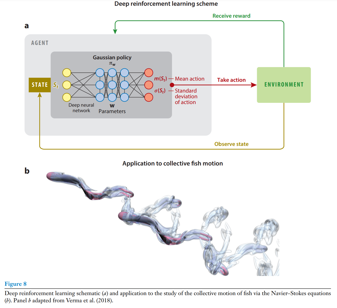
5. 논의와 전망

This review presents ML algorithms for the perspective of fluid mechanics. The interface of the two fields has a long history and has attracted a renewed interest in the last few years. This review addresses applications of ML in problems of flow modeling, optimization, and control in experiments and simulations. It highlights some success of ML in critical fluid mechanics tasks, such as dimensionality reduction, feature extraction, PIV processing, superresolution, reduced-order modeling, turbulence closure, shape optimization, and flow control. It discusses lessons learned from these effoorts and justifies the current interst in light of the technologimal advances of out times. Or goal is to provide a deeper understanding of ML and its context in fluid mechanics. ML comprises data-driven optimization and applied regression techniques that are well suited for high-dimensional, nonlinear problems, such as those encountered in fluid dynamics; fluid mechanics exportise will be necessary to formulate these optimization and regression problems.

ML algorithms present an arsenal of tools, largely inexplored in fluid mechanics research, that can augment existing modes of inquiry. Fluid mechanics knowledge and centuries-old conservation laws remain relevant in the era of big data. Such knowledge can help frame more precise questions and assist in reducing the large conputational cost often associated with the application of ML algorithms in flow control and optimization. The exploration and visualization of high-dimensional search spaces can be simplified by ML and increasingly abundant high-performance computinf resources. 

In the near future, experience with ML algorithms will help frame new questions in fluid mechanics, extending decades-old linearized models and linear approaches to the nonlinear reqime. The transition to the nonlinear realm of ML is facilitated by the abundance of open source software and methods and the prevalent openness of the ML community. In the long term, ML will undoubtedly offer a fresh look into old problems of fluid mechanics under the light of data. Interpreting the ML solutions, and refining the problem statement, will again require fluid mechanics expertise. 

A word of caution is necessary to balance the current excitement about data-driven research and the (almost magical) powers of ML. After all, an ML algorithm will always provide some kind of answer to any question that is based on its training data—data that may not even be relevant to the question at hand. Properly formulating the question and selecting the data, the LM, and its training are all critical components of the learning process. Applying ML algorithms to fluid mechanics faces numerous outstanding challenges (and opportunities!). Although manyfields of ML are concerned with raw predictive performance, applications if fluid mechanics often require models that are explainable and generalizable and have quarantees. 

Although deep learning will undoubtedly become a critical tool in several aspects of flow modeling, not all ML is deep learning. It is important to consider several factors when choosing methods, including the quality and quantity of data, the desired inputs and outputs, the cost function to be optimized, whether the task involves interpolation or extrapolation, and how important it is for models to be explainable. It is also important to cross-validata ML models; otherwise, results may be prone to be explainable. It is also important to develop and adapt ML algorithms that are not only physics informed but also physics consistent, a major outstanding challenge in AI. This review concludes with a call for action in the fluid mechanics community to further embrace open and repreoducible research products and standards. Reproducibility is a cornerstone of science, and several frameworks are currently developed to render this into a systematic scientific process (Barber 2015). It is increasingly possible to document procedures, archive code, and host data so that others can reproduce results. Data are essential for ML; thus, creating and curating benchmark data sets and software will spur interst among researchers in related fields, driving progress. These fluid benchmarks are more challenging than the readitional image data sets encountered in ML: Fluid data are multimodal and multifidelity, they have high resolution in some dimensions ans are sparse in others, many tasks balance multiple objects, and foremost, data come from dynamical systems, where many tasks do not admit postmortem analysis.

We are entering a new and exciting era in fluid mechanics research. Centuries of theoretical developments based on first principles are now merging with data-driven anaysis. This fusion will provide solutions to many long-sought problems in fluid dynamics, first and foremost the enhanced understanding of its governing mechanisms. 

이 리뷰는 유체 역학 관점에서 기계 학습(ML) 알고리즘을 다루고 있다. 두 분야의 접점은 오랜 역사를 가지고 있으며, 최근 몇 년간 새롭게 주목받고 있다. 본 리뷰는 실험 및 시뮬레이션에서 유동 모델링, 최적화, 제어 문제에 대한 ML의 응용 사례를 다루고 있다. ML이 차원 축소, 특징 추출, 입자 영상 속도계(PIV) 처리, 초해상도, 축소 차원 모델링, 난류 폐쇄, 형상 최적화, 유동 제어와 같은 중요한 유체 역학 작업에서 보여준 성과를 강조하며, 이를 통해 얻은 교훈과 기술 발전에 따른 현재의 관심을 논의한다. 우리의 목표는 ML의 본질과 유체 역학에서의 맥락을 더 깊이 이해하는 것이다. ML은 데이터 기반 최적화 및 적용 회귀 기법을 포함하며, 유체 역학에서 자주 마주하는 고차원 비선형 문제를 해결하기에 적합하다. 이러한 문제를 최적화하고 회귀 문제로 구체화하려면 유체 역학 전문 지식이 필수적다.

ML 알고리즘은 유체 역학 연구에서 기존의 연구 방식을 확장할 수 있는 도구로 작용할 수 있다. 그러나 이는 유체 역학 지식과 수 세기 동안 이어져 온 보존 법칙의 틀 안에서 수행될 때 더 효과적이다. 유체 역학 지식은 ML 알고리즘을 유동 제어 및 최적화에 적용할 때 드는 막대한 계산 비용을 줄이는 데 도움을 줄 수 있다. ML은 고차원 탐색 공간을 시각화하고 탐구하는 과정을 단순화하며, 고성능 컴퓨팅 자원의 증가로 인해 그 잠재력이 더욱 커지고 있다.

가까운 미래에는 ML 알고리즘에 대한 경험을 통해 유체 역학에서 새로운 질문을 제기할 수 있을 것이다. 이는 수십 년 동안 지속된 선형화 모델과 선형 접근 방식을 비선형 영역으로 확장하는 데 기여할 것이다. 비선형 ML의 세계로의 전환은 오픈 소스 소프트웨어와 메서드의 풍부함, 그리고 ML 커뮤니티의 개방성 덕분에 더욱 원활해질 것이다. 장기적으로, ML은 데이터를 활용하여 유체 역학의 오래된 문제를 새로운 시각에서 재조명할 수 있는 기회를 제공할 것이다. 그러나 ML 솔루션을 해석하고 문제를 더 정교하게 정의하려면 여전히 유체 역학 전문 지식이 필요하다.

 

현재 데이터 중심 연구와 ML의 '마법 같은' 능력에 대한 흥분을 균형 있게 바라볼 필요가 있다. ML 알고리즘은 항상 학습 데이터에 기반하여 어떤 형태로든 답을 제공한다. 그러나 이러한 데이터가 문제와 연관성이 없을 경우에도 답을 제공할 수 있다는 점에서, 문제를 올바르게 정의하고 데이터, ML 모델, 학습 과정을 적절히 선택하는 것이 중요하다.

ML 알고리즘을 유체 역학에 적용하려면 다음과 같은 주요 도전 과제와 기회가 있다:

• 설명 가능성과 일반화 가능성:
  유체 역학에서는 단순한 예측 성능을 넘어, 모델의 설명 가능성과 일반화 가능성이 필수적이며, 모델의 신뢰성을 보장하는 것이 중요하다.
• 물리학 일관성:
  ML 알고리즘은 물리학적으로 정보를 포함할 뿐 아니라, 물리학적으로 일관성 있는 결과를 제공해야 하며, 이는 인공지능(AI)의 주요 도전 과제 중 하나로 남아 있다.

유체 역학 커뮤니티는 개방적이고 재현 가능한 연구를 더욱 포용해야 한다. 재현 가능성은 과학의 근본적인 토대이며, 이를 체계적 과학 과정으로 정립하기 위한 여러 프레임워크가 현재 개발되고 있다 (Barber 2015).

• 절차 문서화:
  연구 절차를 문서화하고 코드를 보관하며 데이터를 호스팅하여 다른 연구자들이 결과를 재현할 수 있도록 하는 것이 점점 더 가능해지고 있다.
• 벤치마크 데이터 세트 생성:
  ML의 핵심은 데이터에 있으며, 이를 위해 벤치마크 데이터 세트와 소프트웨어를 생성하고 관리하는 것이 중요하다. 유체 역학 데이터는 ML에서 주로 다루는 전통적인 이미지 데이터 세트와는 다르다. 유체 데이터는 다중 모드, 다중 정확도를 가지며, 일부 차원에서는 높은 해상도를 가지는 반면 다른 차원에서는 희소한 경향이 있다. 또한, 많은 작업이 여러 목표를 균형 있게 다루며, 무엇보다도 데이터는 동역학 시스템에서 생성되어 사후 분석만으로는 해결되지 않는 경우가 많다.

우리는 유체 역학 연구의 새로운 흥미로운 시대에 접어들고 있다. 수 세기 동안의 이론적 발전이 이제 데이터 기반 분석과 융합되고 있다. 이러한 융합은 유체 역학의 지배 메커니즘에 대한 심화된 이해를 포함하여, 오랫동안 해결되지 않았던 문제들에 대한 해결책을 제공할 것이다.